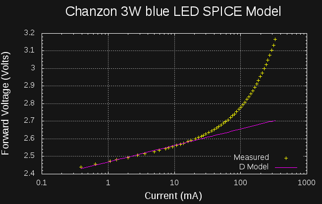
So far, I've put a lot of emphasis on the "analysis" part of the project, and not too much on the "modeling" aspect. So, here's a first cut at creating SPICE models for measured LEDs (or other diodes). As I mentioned at the start, the system only collects enough information to calculate parameters for DC (or low-frequency transient) SPICE simulation. I've come up with a method for estimating these parameters that seems fairly robust and produces very usable results. Here's an example of the model compared with actual data points measured for a Chanzon 3W blue LED:

In this case, the data points were only collected up to about 350mA, but within that range, the fit seems very good; certainly good enough to run SPICE simulations (which should always be viewed with suspicion, anyway).
Approach
I've written code to model diodes from measurements on three (or maybe four) occasions over the years, and have found two things to be generally true:
- Non-linear fitting with the Levenberg-Marquardt (LM) algorithm can give excellent results
- LM fails to converge on diode models frustratingly often
The only cure I have found for the convergence issues is to ensure the starting "guess" supplied to the algorithm is close enough to the solution. Of course, this sounds like a chicken-and-egg problem, but the answer turns out to be fairly simple - a linear model can be initially fit (without convergence concerns), then used to initialize the non-linear optimizer.
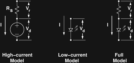
The fitting actually takes place in three stages, corresponding to the three models shown here:

The "Full Model" is the ultimate goal, and represents the DC diode model used by SPICE. In this model,
the internal series resistance of the diode is explicitly modeled. The total voltage across the diode (including the resistance) is based on the current, and is modeled by:
The first term is just a re-arrangement of the Shockley diode equation, and the second term is Ohm's law applied to the series resistance. There are three unknown parameters in this model, namely:
- Is, the diode reverse saturation current
- n, the diode ideality factor
- Rs, the series resistance
Vt, the thermal voltage ( = kT/q), is approximately 26mV at room temperature, and is assumed constant for all the data points - see below for more details.
High-Current Model
The first step of the algorithm is to model the diode as a fixed voltage in series with the internal resistance. For large currents, the second term (IRs) dominates the forward voltage, and the diode voltage is approximately constant. This is the regime in which we would say that a 1N4148 diode has a 0.7V forward voltage (ignoring current), for instance. The algorithm uses high-current data points to fit a simple linear model producing an estimate of Rs and (the fixed value) Vd. The following plot shows the high-current model for the blue LED shown above:

Low-Current Model
The next step in the algorithm is to estimate the values of n and Is using the low-current measurements. The LM algorithm is used to fit the first term in the above equation, initialized with a value of 1.5 for n (which is almost always between 1 and 2), and an initial Is value derived from the fixed "diode voltage" found in the high-current model. Fitting this simpler model with a good initial guess seems to be fairly robust. Here is the result (shown on a log current scale) for the estimated low-current model for the same blue LED:

Full Model
The two initial models provide decent estimates of Is, n, and Rs, which are then used as starting guesses to initialize the LM algorithm for optimizing all three parameters simultaneously. In practice, this procedure seems to work pretty well; I've tried it on 16 different LEDs so far, and it has always converged, and produced good-fitting models.
One more trick is used to facilitate convergence. The number of points used for the two initial estimates are varied in a loop, and the result with the lowest overall error is used. Typically, most initializations converge to exactly the same final values.
SPICE Modeling
Here's the resulting SPICE model for the above LED:
.MODEL chanzon_3W_blue D(Is = 1.504091e-34,
+                        n = 1.336514e+00,
+                        Rs = 1.510662e+00)
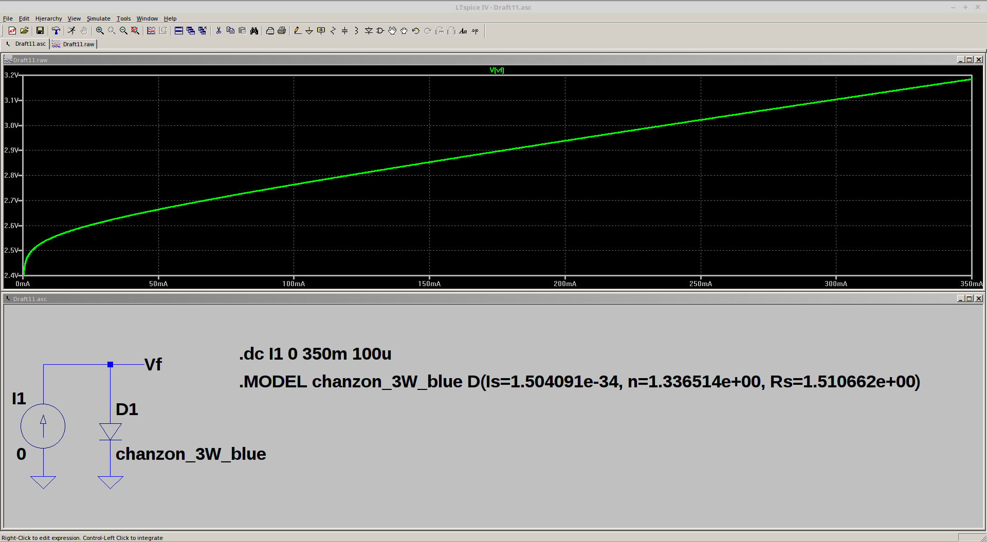
And how it simulates in LTspice:

The result, as expected, matches the measured points very closely. Interestingly, the series resistances for all the LEDs I have measured have been around 1 ohm (here 1.5), which validates the choice of Kelvin sensing connections to the LED; without the four-wire arrangement, measuring this small resistance accurately would be impossible.
Temperature Effects
I don't (yet?) have a good way to measure the LED temperature as the data points are being collected. The LED temperature at high currents is certainly higher than that at low currents, which effects both Is (strongly) and Vt (weakly), so assuming these are constant for all the data isn't strictly correct. However, if you intend to use the LED under the same conditions it was measured in (same heatsink, airflow, etc), the temperature will be roughly the same, and the model will remain valid. If this really matters to you, you should probably measure your LED in situ to eliminate these effects.
Shut Up And Show Me The Code, Already
I initially developed the algorithm in octave using the leasqr() function for the LM optimization, then ported it to Python using scipy.optimize.curve_fit(). The two programs give essentially identical results.
The octave code is a mess, but the Python ain't bad. I've checked it in to the the GitHub repo.
 Ted Yapo
Discussions
Become a Hackaday.io Member
Create an account to leave a comment. Already have an account? Log In.