Low pass filters are often used to reduce higher frequency components of a signal. Electronic LP filters are for example used after a sensor to remove high frequency noise from the signal before analog to digital conversion in a micro controller. Often we then want to reduce the bandwidth of the signal even more using a digital LP filter within the micro controller program.

An equation for the calculation of a first order digital low pass filter can be written as

y(k)= y(k-1) (1-a) + ax(k)

or, after a little rearrangement

y(k)= y(k-1)  - a y(k-1)  + ax(k)

where y(k) is the new filter output value calculated from the old output value y(k-1). k is the sample number and the new input value from the AD converter x(n) and a coefficient a. This filter has short memory, we only use the present and previous sample values.

If a is set to 0, the new output will not change at all. If equal to 1 the new value will be equal to the new input value only. For a between 0 and 1 this equation will mix a part of the new value with a part of the old value and in this way act as a low pass filter. A larger value of a will weigh new input values more than the old output and the filter will thus react faster. The value of a determines the filter bandwidth or in other words the time constant. If the input x is constant the output will approach this value.

The filter equation is simple and fast to calculate if we have a controller with a floating point processor. But if we use a simpler controller we are stuck with integer arithmetic or a very slow floating point library. I will use integers for the following description.

Assume a 10 bit A/D converter. The value range of  x(k) is then 0 - 1023. The coefficient a is smaller than 1, say 0.1. The result of a x(k) will then be in the range 0-102. We see that most of the precision we had from the 10 bit converter is severely reduced. We can remedy this by scaling the equation.

Scaling

We want to maintain the resolution we had from the converter by multiplying the equation by a constant b=1/a. We then get

b y(k)= b y(k-1) - y(k-1) + x(k)

Instead of reducing the input values we now maintain a corresponding larger y(k) value. To get the correct output the filter output must then be divided by b. We can also write this as

z(k)= z(k-1) -  z(k-1)/b + x(k)

where the new variable z= b y. The above implies both multiplication and division, both costly operations even when using integer arithmetic, and some simple controllers don't even have a 8 by 8 multiplier.

Instead of a standard multiplication I will therefore chose b=2^m, that is 2, 4, 8 and so on. This will limit the possible bandwidths we can get but also reduces the multiplication and division to simple  left and right shift operations. Shift operations are fast on any processor.

z(k)= z(k-1) - z(k-1)>>m + x(k) 

or equivalently as a C program statement

z= z - z>>m + x;

and the filter post processing to scale from z to y

y(k)= z(k) >> m

Let's assume the 0-1023 input range from the AD converter as before and m=6. Then b=64 corresponding to a=0.0156. The filter output range is 1024*64=0-65535 which can be maintained in a 16 bit unsigned integer variable. However, watch the sequence of operations: first do the  z(n-1) - z(n-1)>>m and then add x(n), if done in the opposite way, the  z(n-1)  + x(n) can overflow the 16 bit variable.

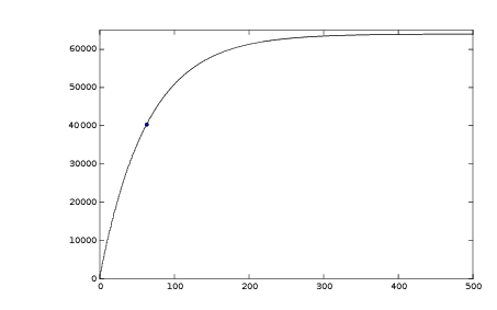
The graph shows the step response of this filter with m=6 and  x=1000. The steady state value of z is  1000*64=64,000. First order step responses pass the time constant at 63%= 40,300. That is at about the 64th sample. If the sampling time is 10 msec, this corresponds to a time constant of 640 msec..

By operating with shifts instead of a real multiplication the freedom to chose filter time constant is limited to a few values. On the other hand, first order filters are fairly dull and the exact bandwidth is usually not important. But we can increase the offered time constants a bit by introducing an extra shift operation.

Non-integer shifts

I now introduce a new shift operation, n shifts this time.

z(k)= z(k-1)  - z(k-1)>>m - z(k-1)>>n + x

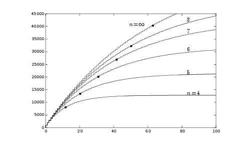
The effective shift is now p= lb(2^-m + 2^-n), where lb is the binary logarithm. By playing with m and n we get a large repertoire to choose from. As an example, still with m=6 we get these values:

n	p	b= 2p	z steady state value
4	3.68	12.8	12,800
5	4.41	21.3	21,300
6	5	32	32,768
7	5.41	42.7	42,700
8	5.68	51.2	51,200

The step responses for these values of n are graphed here. The dots indicate the time constant for each filter, at the step number close to b.

We can add shift operations to increase the resolution of the time constant even more. But as we do so we approach multiplication, which is a sequence of shift and add. And that was not the point.