Johannes
-
Schematic diagram - first drafts
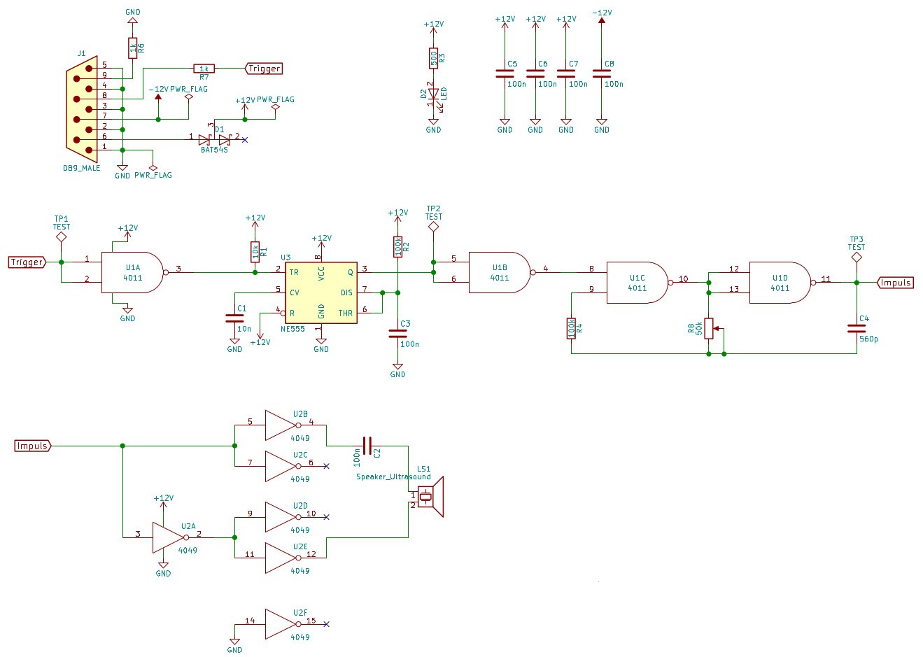
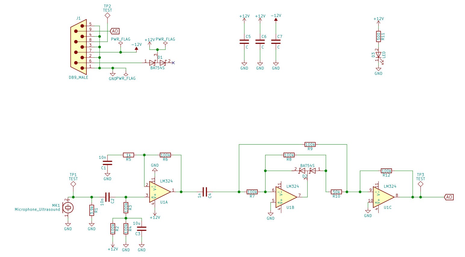
07/05/2018 at 16:42 • 0 commentsI chose ultrasonic transmitter MA40S4S and receiver MA40S4R. In the German data sheet there are many application notes with many examples of schematics. I did not find these documents in English though.
The following diagrams were created with KiCad/Eeschema based on the data sheet.
![]()
![]()
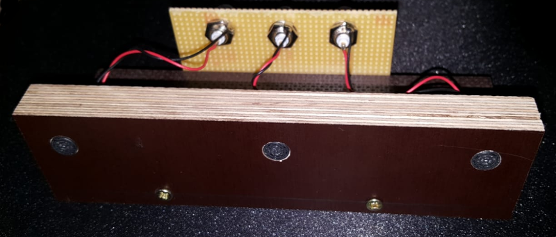
My plan is to build sub-modules that transmit and receive. Both use the same interface, which will also be used by a measurement-device. For this device all I have so far is a vague concept which I will refine in a future post:
- maybe a box with several interfaces (minimum of four) for connecting sub-modules, which
- output the 'burst*
- analogue input from three sensors
- ADC for said analogue inputs. maybe a 1 bit ADC (aka schmitt trigger)
- inside some kind of digital signal processor. may even be a small 8 bit µC
- output of scanned image. maybe a display or connector for a computer which runs 'display software'For now I will focus on creating some sub-modules and test them with an oscilloscope.
Ideally this will allow me to test my concept (in 2D for I only own a two channel oscilloscope right now).
-
Theory of operation pt. 2
06/27/2018 at 16:53 • 0 commentsIn the previously post I described an simplified version of the scanning array with only two sensors.
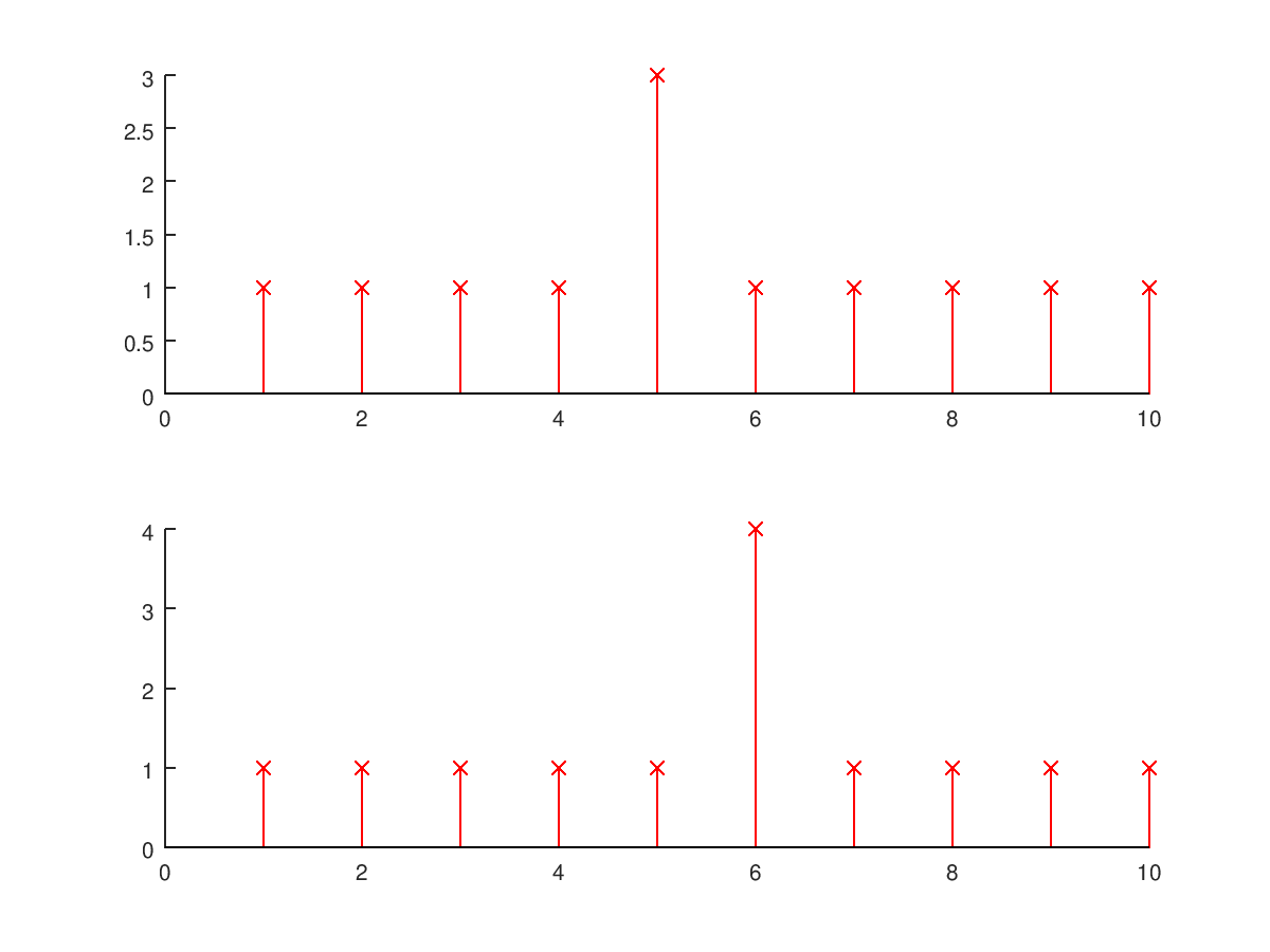
This is, what the signals would look like if there was a single object.
![]()
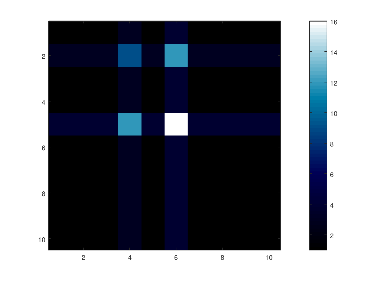
Well, what's next? With these time-discrete readings of ultrasonic amplitude we can do something simillar to a time-discrete convolution to create a 2D image.
![]()
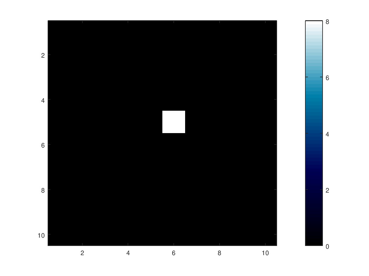
The white dot marks the object. In this simulation there is only one object, if there were more than one, artefacts will appear.![]() To eliminate the artefacts, a threshold is applied.
To eliminate the artefacts, a threshold is applied.![]() There is another artefact. The white dot is an area where the setup cannot detect objects due to shadowing. For now this cannot be eliminated.
There is another artefact. The white dot is an area where the setup cannot detect objects due to shadowing. For now this cannot be eliminated.
Here is the octave script, I used to create the images.%input data simulation: clear size = 10; f=ones(1,size); g=ones(1,size); style='rx'; f(2)=3; f(5)=4; g(4)=3; g(6)=4; threshold = 4; %plot input data subplot(2,1,1) stem(f,style) subplot(2,1,2) stem(g,style) %create heatmap z = zeros(size, size); for r = 1:size for c = 1:size z(r,c) = f(r)*g(c)-threshold; end end z(z<0)=0; %plot heatmap fig = figure; colormap('ocean'); imagesc(z); %create plot colorbar; %intensity bar -
Theory of operation
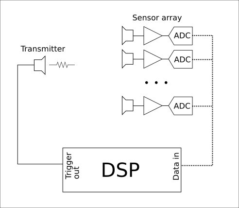
06/26/2018 at 21:46 • 0 commentsThis is an overview of the main function.
![]()
The main part is a digital signal processor, which creates the ultrasonic burst. The Signal is send out by the transmitter, reflected by an object and received by the sensor array.
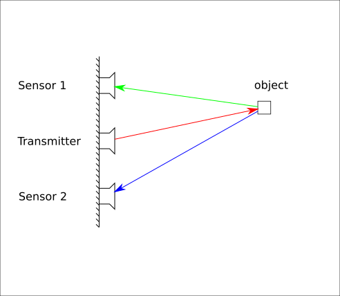
I will focus on 2D scanning at first. Therefore the sensor array only consists of two sensors, aligned in a row with the transmitter. This also simplifies the required calculations for object detection.
![]()
In this first prototype sensor 1 and 2 are 160mm apart, the transmitter is located in the middle between the sensors.![]()
-
First note on this project
06/26/2018 at 16:46 • 0 commentsCredits for the background image go to LiDAR ParaView which is released under Creative Commons Attribution License 3.0, until I am able to provide my own images.
The picture is an example of the result which I try to create with this 3D scanner.
Ultrasonic 3D scanner
This project's goal is to gather 3D images via ultrasonic distance measurements and a sensor array.
 To eliminate the artefacts, a threshold is applied.
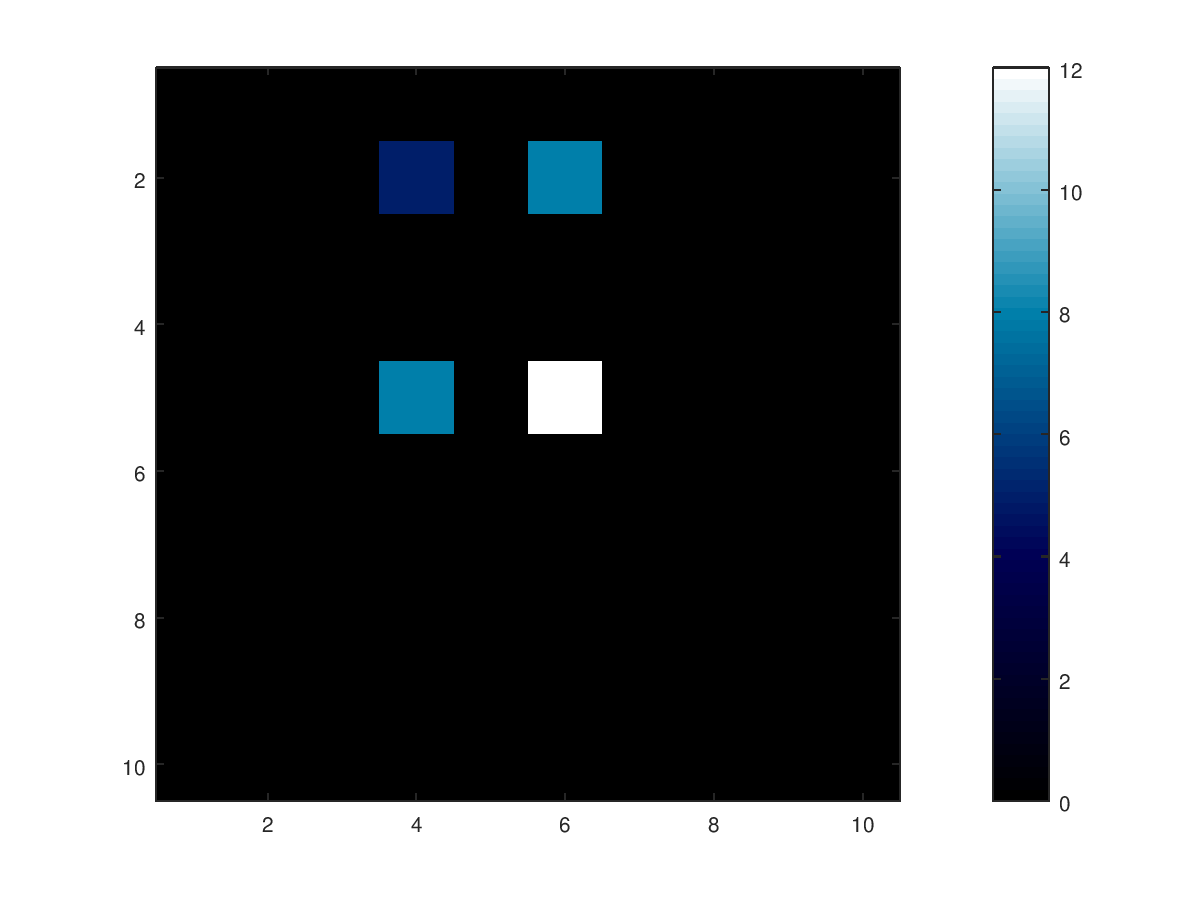 There is another artefact. The white dot is an area where the setup cannot detect objects due to shadowing. For now this cannot be eliminated.