With the freezer in the garage and the control system operating I started the next phase of the project:  system modeling.

I filled the carboy with 26.9 kg of tap water.  I then placed a temperature probe in the thermowell within the carboy, a temperature probe on the wall of the freezer and left a temperature probe out external to the freezer.

I then recorded four data files: Twice with the freezer cooling the carboy and twice allowing the carboy to warm up. 

The model that I developed for the system is below.  It is an “electrical equivalent” model representing heat transfer between the ambient environment, the freezer and the carboy.  (Note the funny symbol for q is a current source pointed away from Tf to ground.)

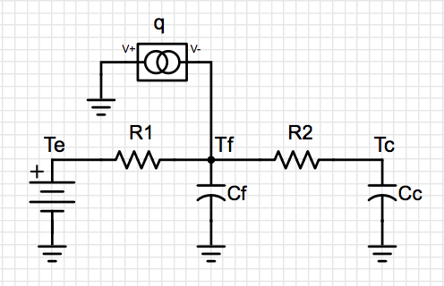
Cc is the heat capacity of water in the carboy.

Cf is the heat capacity of the freezer.

q is the heat collected by the freezer.

R1 is the thermal resistance between the freezer and the ambient external environment.

R2 is the thermal resistance between the freezer and the carboy.

Te is the ambient external temperature.

Tf is the temperature of the freezer wall (measured from the inside of the freezer).

Tc is the internal temperature of the carboy.

The differential equations for the model are below.

By measuring Tc, Tf and Te I was able to calculate Cc, Cf, q, R1 and R2.  (I used Matlab and Simulink to run the simulations (version r2017b).  I am more than happy to upload the files for others to use if interested.  Matlab now offers a "hobby" edition of the matlab software for about $45.  Add on modules such as simulink are an additional $45.  I think they have been watching everyone migrate to Python.)

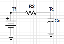
First I simulated the carboy temperature using the freezer wall temperature I measured.  This let me simplify my model to only R2 and Cc.  I assumed a Cc of ~50000 J/C using a specific heat of 4.18 kJ/(kg C).  I was then able to tune R2 so that when simulating Tc using Tf, R2 and Cc my simulated Tc match the measured Tc.  The simplified model is below.

Cc = 50000

R2 = 0.65

The simulation results and images of my simulink models are below.

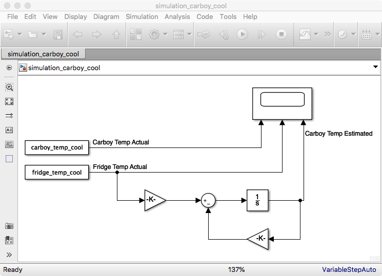
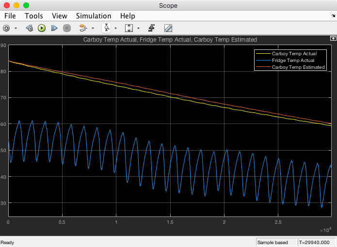
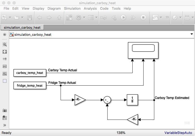
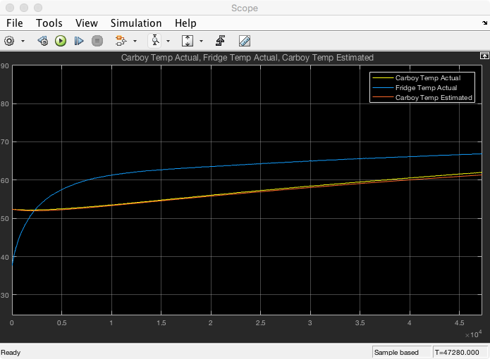
As you can see the simulated Tc matches the actual measured Tc very closely.  The time axes is in seconds.

I then setup a simulink model for the larger system with Te and q as the inputs.  I then tuned the values for R1, Cf and q to align my simulation with my the measured Tc and Tf.  Results from the simulation are below.

R1 = 1.6

Cf = 5000

q = 156*pwm_percentage

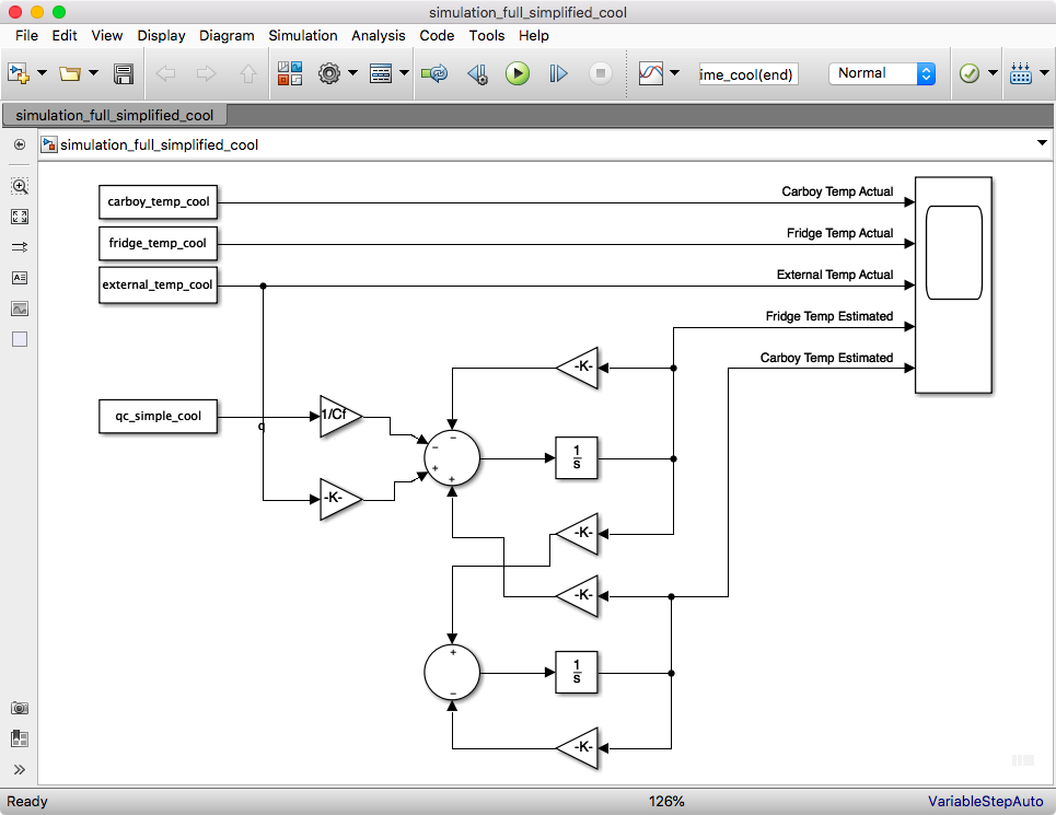
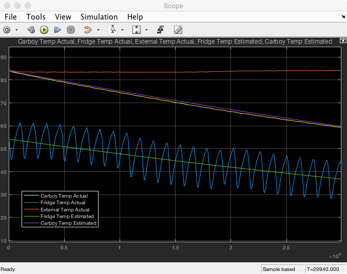
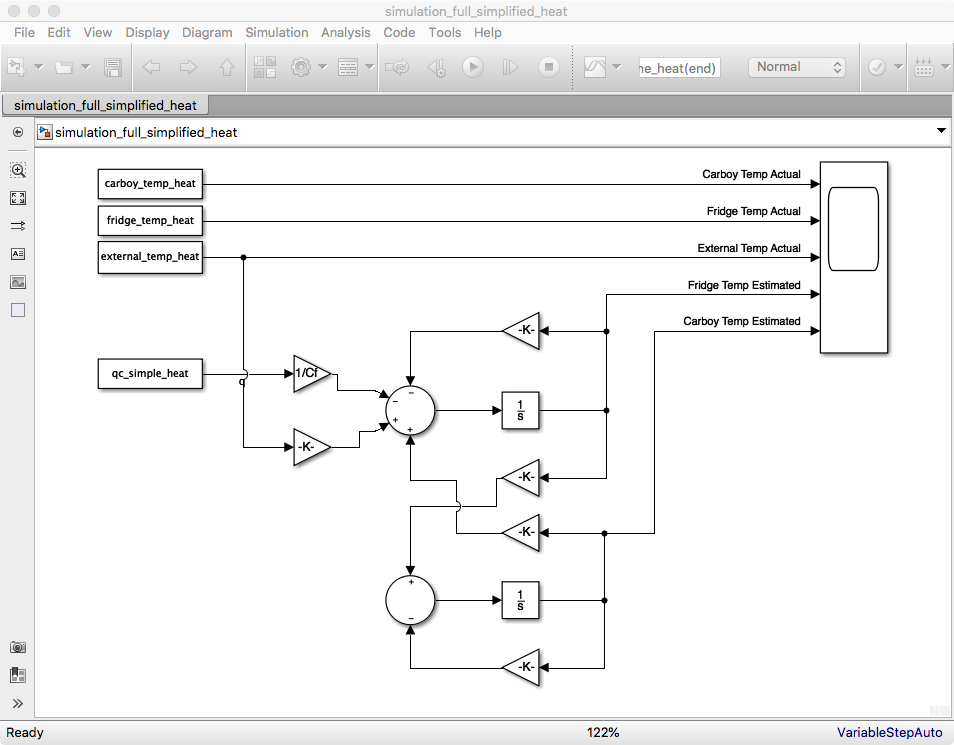
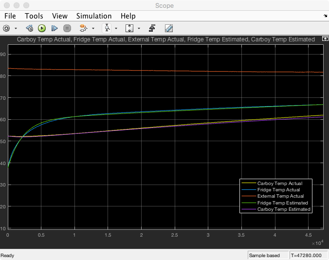
It works!  It is very exciting again!  I finished all this work over the weekend and then did a little dance around the table.  I also noticed that my wife is very impressed with milestones in my projects.  She usually celebrates with some eye rolls and “that is vey nice honey” statements.  I take that as high praise indeed!

Next time update I should be able to provide feedback on development of my state space closed loop control algorithm!  (Also very exciting!)