The Idea: Restate and test MILP model for determining the parameters of the clap algorithm.
With the help of GNU Glpk and PyGlpk, the mixed integer linear programming (MILP) model that was described in the last several logs has finally been implemented! And, in doing so, several issues with the original model were discovered and fixed. The prior logs on the system model may even be removed in the future. However, in attempt to reduce the amount of time spent writing these logs, many of those details are glossed over here; writing these logs take a significant amount of time, unfortunately. Instead, much of the model is simply restated in this log. In addition to the restating the model, this log includes a brief example demonstrating the model works as intended. The example and the respective Python code can be found in the project's repository!
And, like the last log, the equivalent inline latex is used to refer to the symbols presented in the images. Hope this isn't too confusing!
The Theory: Model description.
The signal $x_n$ represents the sampled audio.
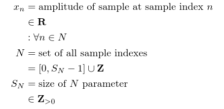 The clap that needs identification is defined as a sudden spike in the energy of $x_n$, where each energy $e_m$ is defined over a small interval.
 A spike in energy can be regarded as a sudden increase in energy over a period, and then a sudden decrease over another period of time. The sudden changes are signified by either the energy $e_m$ exceeding the threshold $e_H$ or falling under the threshold $e_L$, for their respective durations.
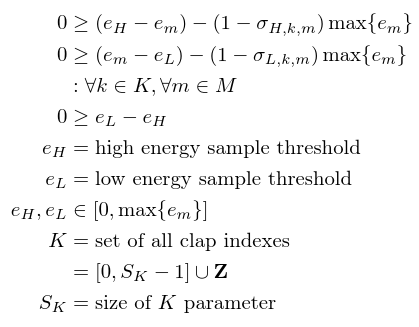 $\sigma_{H,k,m}$ and $\sigma_{L,k,m}$ are both indicators that represent the aforementioned durations. Specifically, $\sigma_{H,k,m}$ represents the duration for which $e_m \ge e_H$ is true for each clap $k$.
 The three unknowns are $\Delta m_k$, $\Delta m_H$, and $\Delta m_{H,k}$. $\Delta m_k$ represents the amount of time---measured in samples $m$---between each clap $k$. $\Delta m_H$ is the minimum amount of time $e_m \ge e_H$ needs to be true for clap $k$. $\Delta m_{H,k}$ allows $e_m \ge e_H$ for clap $k$ to be true longer than $\Delta m_H$. And, since it's probably not very clear, assume $m_{L,UB,-1} = 0$.
Next, $\sigma_{L,k,m}$ represents the duration for which $e_m \le e_L$ is true for each clap $k$.
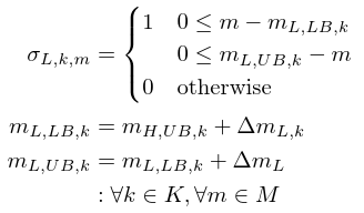 The unknowns are $\Delta m_{L,k}$ and $\Delta m_L$. $\Delta m_{L,k}$ for clap $k$ allows $e_m$ to fall in between $e_H$ and $e_L$ before $e_m \le e_L$ needs to be true. Similar to $\Delta m_H$, $\Delta m_L$ is the minimum amount of time $e_m\le e_L$ needs to be true.
In order to progress with this explanation, consider the following definitions.
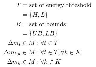 Assume the domain of variables that begin with $\Delta$ are $M$. With these definitions, the indicators $\sigma_{H,k,m}$ and $\sigma_{L,k,m}$ are reduced to a single indicator.
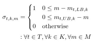 To further simplify, $\sigma_{t,k,m}$ is true if and only if the conditions $0 \le m - m_{t,LB,k}$ and $0 \le m_{t,UB,k} - m$ are true. Taking advantage of the if-then constraint, the aforementioned conditions are represented with the following.
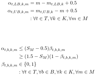 The conditions $\beta_{t,LB,k,m}$ and $\beta_{t,UB,k,m}$ are further simplified with a logical-AND operation. The result is $\sigma_{t,k,m}$.
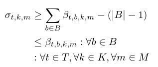 Finally, the objective is to find the values of the unknowns that maximize the difference between $e_H$ and $e_L$. The variables that need solving are the following.

The Implementation: PyGlpk and GNU Glpk
For those who have seen the logs on the embedded systems project, GNU Glpk has already been used in other projects as a way to solve LP models, albeit the application was for flow-network problems. Instead of the LEMON Glpk interface as described in the embedded system logs, the presented MILP model is solved with Glpk via the PyGlpk interface. As stated earlier, the source code of the first completed version can be found in the project's repository. There will be one more version of the source code since the current model does not take into consideration multiple sets of audio signals ( and the source code is somewhat messy, admittedly ).
Let's start with a simple example! Consider the following signal.
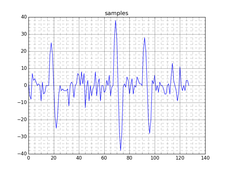
The signal presented above is actually computer generated with a Python script found in the repository. Before moving on to the real thing, debugging and testing is simpler to do with a simpler signal. The signal itself is created by first sampling from a normal distribution and then adding sine waves which represent the claps. As one can hopefully tell, there are 3 claps added to the noise.
With a $\Delta n = 4$, the signal is converted to the following energy samples.
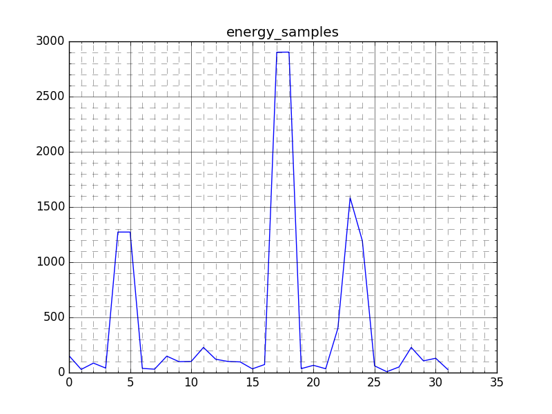
Experimentation reveals that a small $\Delta n$ is highly desirable, mainly due to the assumption that an actual clap duration is quick relative to other sounds. But, if $\Delta n$ is too small, there are sometimes unwanted "dips" in the energy signal. In order to fix this problem, a new definition of energy will be considered in a future log.
Another revelation is that modifying the bounds on certain variables can drastically reduce the amount of time needed for the optimization. For instance, since from the figure it is clear that $\Delta m_{H,k}$ for every clap $k$ should equal 1, setting the bounds of $\Delta m_{H,k}$ to 1 reduces the search space and thus saves a lot of optimization time.
( I know this probably very obvious, but the thought didn't really occur to me until I started experimenting with the model. )
| Variable | H | L |
| e_t | 1194 | 121 |
| Delta m_t | 1 | 2 |
| \max\{ \Delta m_{t,k} : k \in K \} | 0 | 7 |
| \max\{ m_k : k \in K \} | 3 | 3 |
Additionally, the bounds for the duration are presented below.
| m_{t,b,k} | m |
| m_{H,LB,0} | 4 |
| m_{H,UB,0} | 5 |
| m_{L,LB,0} | 12 |
| m_{L,UB,0} | 14 |
| m_{H,LB,1} | 17 |
| m_{H,UB,1} | 18 |
| m_{L,LB,1} | 19 |
| m_{L,UB,1} | 21 |
| m_{H,LB,2} | 23 |
| m_{H,UB,2} | 24 |
| m_{L,LB,2} | 25 |
| m_{L,UB,2} | 27 |
Didn't really take the time to generate the plots with lines indicating where the bounds are. But, a quick comparison of the bounds and variables with the figure suggest the results at least appear to make sense! For now, let's call it quits on this log...
The Conclusion: Final observations and plans for next log.
The optimization takes a while to run. It might be worthwhile to adjust the objective such that any plausible solution is determined. The next and hopefully final version of the model will include a different definition for energy. This new definition will include some overlap since it was discovered through experimentation of the a real audio signal the duration of each clap is extremely quick compared to the sample rate of the microphone's ADC. Filtering may also be considered but it may not be necessary if the new definition of energy works out well enough.
 andrew.powell
Discussions
Become a Hackaday.io Member
Create an account to leave a comment. Already have an account? Log In.