Programmable Precision Resistor

Just a quick follow-up on this project. Today I switched the unit on and after a briefly turning on it shut off again, completely dead. I checked the fuses - all fine. So I had to open the case and I was presented with the smell of burnt components - but nothing really visible.

The only logical explanation: Either the DC/DC converter or the inrush current limiting resistor must have gone (or both, obviously). My money was on the inrush current limiting resistor and sure enough it reads >2 MOhms. No burn marks though. At closer inspection I found that I used an unsuitable resistor: It has a flame-proof coating, but the datasheet does not mention that it is surge/pulse rated. Oops! 

Also, the schematics showed a 33 Ohm resistor, which is a copy & paste error. I actually used a more appropriate 12 Ohm resistor - with 33 Ohms the power dissipation is needlessly high, especially at 120V. Now I have to order a more appropriate replacement...

I didn't really think about the BOM cost of my programmable decade resistor until I was asked. Then I also wanted to know. It is fairly difficult to put a number to what I paid, since I had a lot of components left from other projects that I could use. This includes not only cheap chip resistors and MLCCs, but also connectors, the microcontrollers etc.

Normally, I order my parts from mouser and digikey. For some of the industry-standard components, connectors etc. I also use local distributors (cheaper!). This is why I'll only give a very rough estimate for the per unit costs including taxes (and not including any shipping costs). For some of the parts like the PCBs there is a minimum order quantity that will increase the cost in most DIY scenarios.

Mechanical parts

Mainboard

UI Board

Power supply board

Conclusion

According to this calculation the total cost of the unit would be about 369 €. Quite a lot, actually. This doesn’t necessarily reflect what I paid for it though. One example: I bought 5 NE-18 type switches on ebay for about 2 € each. These are not necessarily the same as the ones provided by mouser, but both variants could be used.

I was asked a few times how I did the front and rear panels, so this is what I’d like to talk about in this blog. There are different ways to achieve a similar result. For me, the easiest and most cost-effective solution was to just design another PCB – I know how KiCAD works and it does everything I need it to do.

The basics

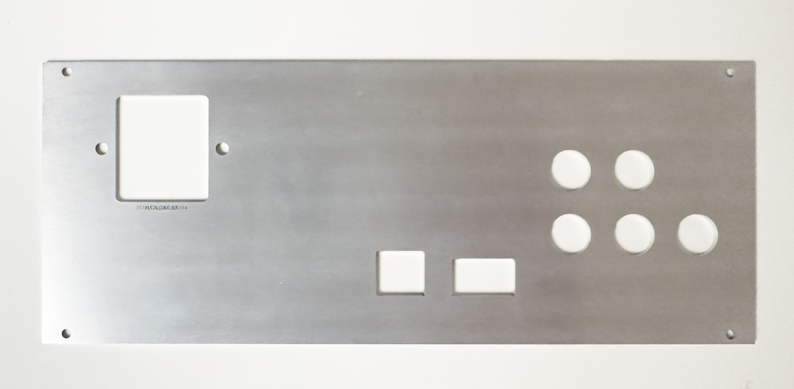
Depending on the actual use case you can use a regular FR-4 board. For this project, however, I chose an aluminum PCB. Those only have one copper layer and the prototyping service might (and probably will) specify different limits/process parameters. But other than that it is very similar to designing a regular PCB.

The first question might be which side of the PCB shall be visible. For this I chose the top side, i. e. the side where the copper layer would be. This allows me to remove the solder mask from the bottom, exposing the bare aluminum (again: This is a one layer PCB). Now the aluminum part makes good electrical contact with the case, so that it can be grounded properly (safety) and work as a shield.

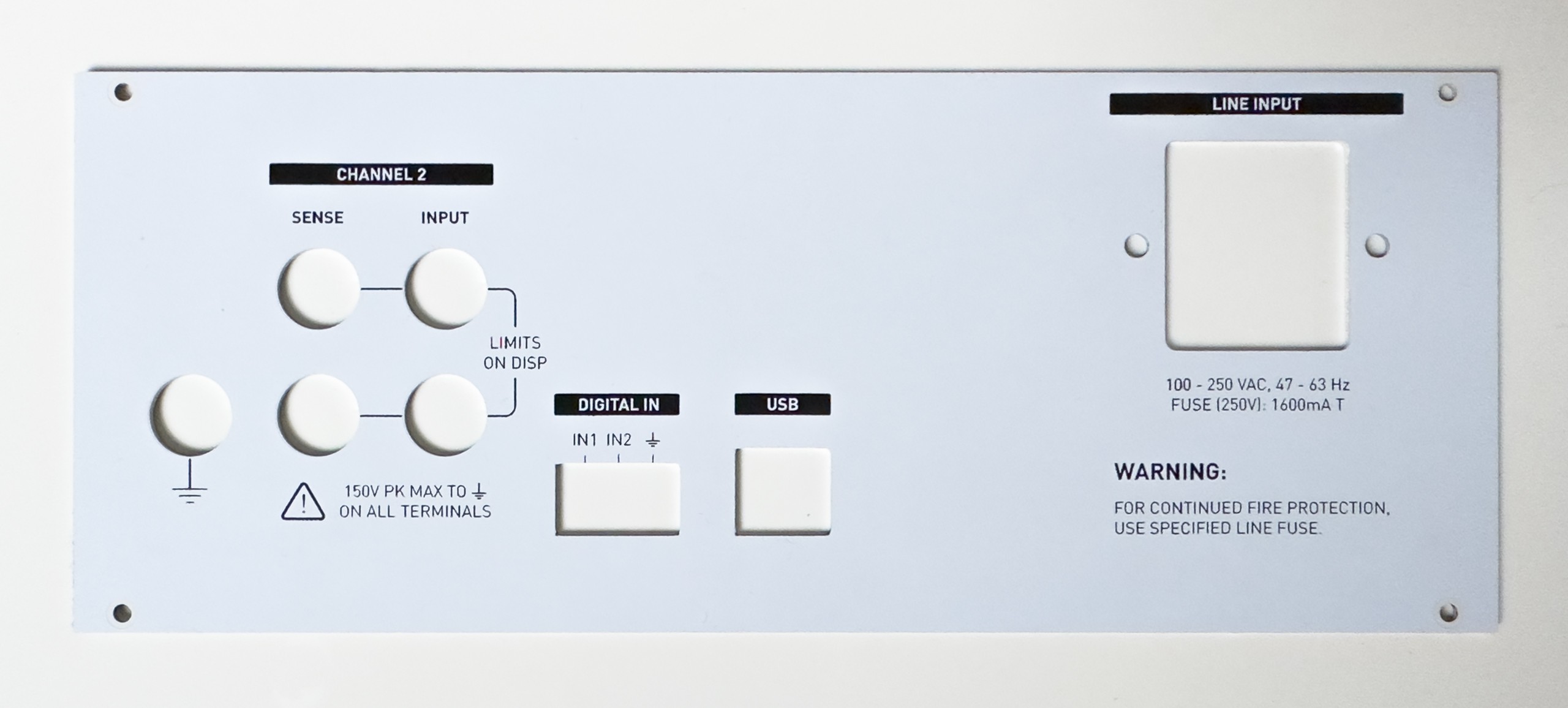
Then I removed the copper layer (almost) completely, because I didn’t want to risk having a large floating conductor anywhere*. The solder mask, however, stays in place, giving the front panel its white color. The (black) silk screen is perfectly suitable to group and label the controls, connectors etc. In theory you could remove the solder mask partially on the front panel as well, exposing the aluminum to give you a fourth color. If you decide not to completely remove the copper, but expose it instead, you have the option for a fifth color. Whether this is a good idea is up to you.

*) At this point it probably wouldn’t really matter which side you use for the solder mask and silk screen I think

A few tips

If you plan to use certain components over and over again, maybe for different projects or maybe just because you have 20 switches of the same type on your UI board, it might be really handy to create a footprint for the cutout, labels, graphics etc. The same is also true for the outline of the panel itself. Most of my projects use the same cases, switches, power connectors etc. over and over again – so creating the footprints is what I did.

In some use cases you might find helpful to place symbols on a schematic and import the footprints based on the schematic. In most cases this would be overkill though – simply adding the footprints to the PCB (in Pcbnew) does the job equally well.

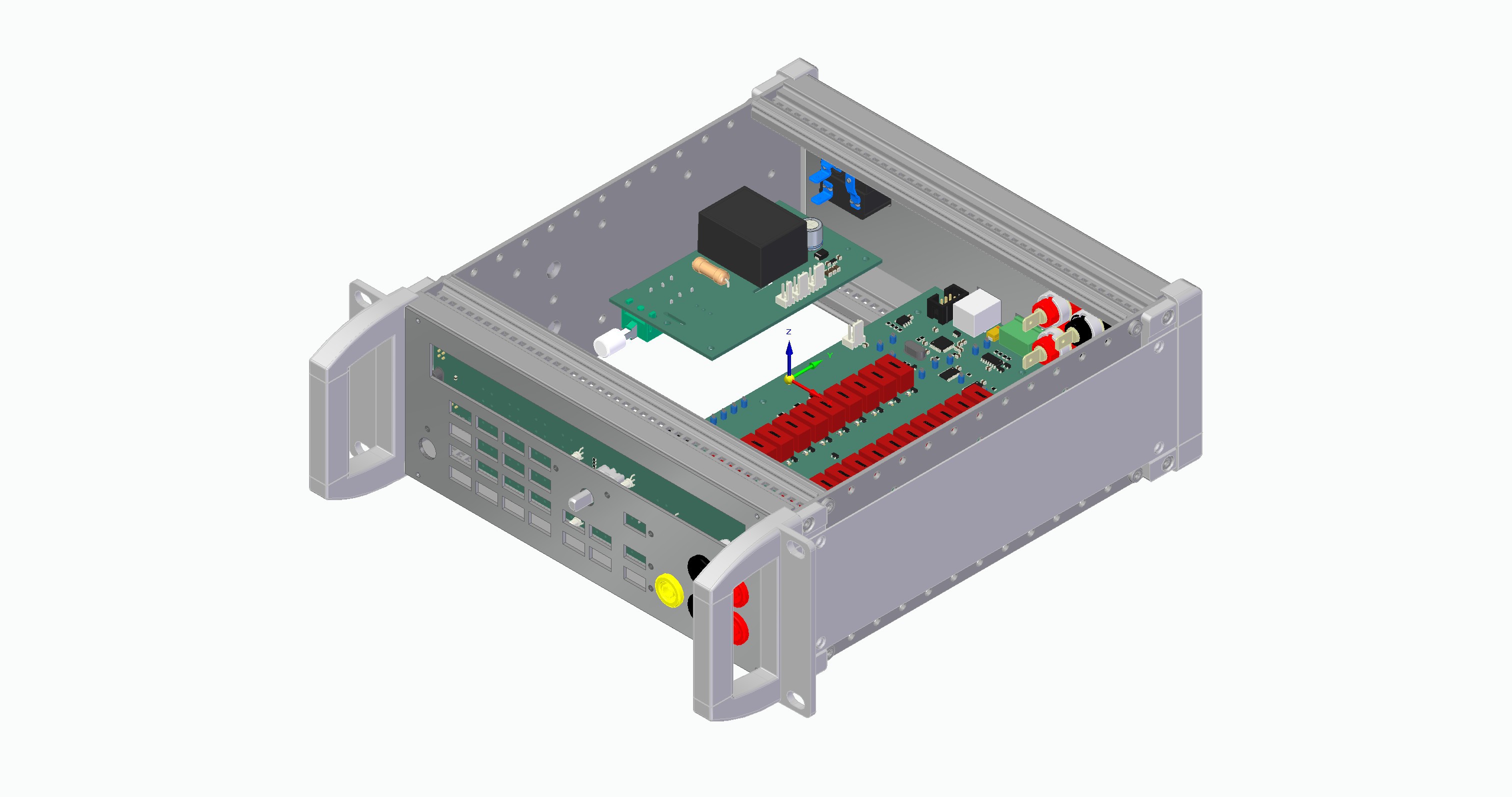
Many case and component manufacturers provide 3D models on their websites that can be combined into an assembly with all the panels and PCBs to catch errors early on. Unfortunately, there is no 3D model available for the switches I used and I couldn’t be bothered to create them myself. Still, this approach helped me to avoid some issues with the front panel that would have required a second revision otherwise – now the first revisions of both the front and rear panels worked perfectly.

The design

The layout of the user interface etc. depends on the application and is completely up to you – obviously. The labeling, the fonts, additional graphics and so on can improve or hurt the usability significantly. So it’s usually a good idea to spend quite a bit of time thinking about how you and more importantly any other operator should or would likely use the device and make it as easy to work with as possible. It can be helpful to go through a few iteration on paper (or any suitable program) before even starting the implementation in your PCB software.

Also it’s really helpful to take some inspiration from the designs of big TME manufacturers like HP/Agilent/Keysight, Keithley, Tektronix & co. You don’t have to copy them, but adopting some of the general concepts they use might get you started more quickly and may result in a more professionally look and feel.

After being asked about some aspects of the mechanical design and components used a few times, I'd like to address those questions. I have to admit that I'm neither very good at the mechanical design, nor do I have a 3d printer (yet) or a shop where I can do metal work myself. That being said, I was still able to design a reasonably professional looking device and bring it to life with the help of modern prototyping services.

The new 3D printed knob for the rotary encoder.

Next steps

There will be a separate post where I explain the fairly straight forward process of designing the front and rear panels.

After the modification described in the previous log I let the “adjustment” and calibration procedure run again. 5 days later I repeated the calibration (without doing the adjustment). As before, all measurements are performed with an Agilent 34401A 6.5 digit multimeter.

Accuracy of the resistance

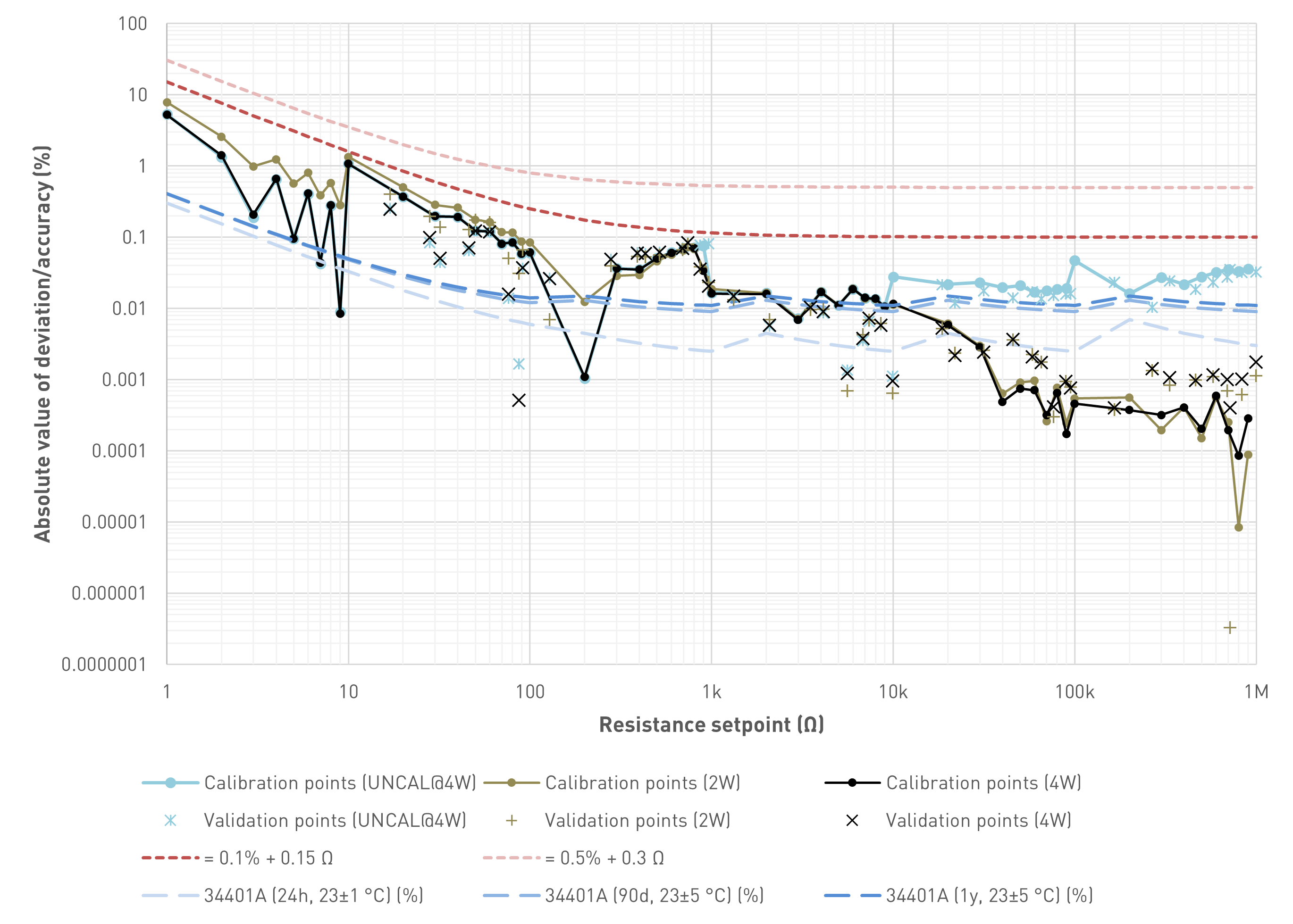
First up is a diagram that shows the absolute value of the deviation of the measurement from the setpoint. The tested values are grouped as follows:

• Calibration points: There are 55 calibration points (0 Ω, 1 Ω, 2 Ω, .., 9 Ω; 10 Ω, 20 Ω, .., 90 Ω; 100 Ω, 200 Ω, .., 900 Ω; 1 kΩ, 2 kΩ, .., 9 kΩ; 10 kΩ, 20 kΩ, .., 90 kΩ; 100 kΩ, 200 kΩ, .., 900 kΩ). In the diagram, all calibration points are connected via lines for visual purposes only. This does NOT imply that we can estimate the deviation for setpoints between two calibration points by looking at this line.
• Validation points: These are 9 randomly selected values per decade for the upper five decades. All values of the first decade are already included in the calibration points. This results in 45 additional points. Validation points are not connected by a line.

The diagram includes curves for the following scenarios:

• UNCAL@4W: The programmable resistor is used in its uncalibrated mode, where the user selectable setpoint equals the hardware setpoint. If, for example, the user enters 130 kΩ, the 6th decade would be in the 100kΩ, the 5th decade in the 30kΩ and all other decades in the shorted position. Also, the display logic ignores the calibration constants and shows 130.000 kΩ. (The input LED switches to red in order to indicate the uncalibrated mode.) For the diagram shown, the measurement was performed using a four-wire resistance measurement
• 2W: In the calibrated two-wire mode, the programmable resistor uses the two-wire calibration constants to optimize the hardware setpoint so that the actual resistance value is as close to the setpoint as possible. The calibration in this scenario is also performed using two-wire measurements
• 4W: In the calibrated four-wire mode, the programmable resistor uses the four-wire calibration constants to optimize the hardware setpoint so that the actual resistance value is as close to the setpoint as possible. The calibration in this scenario is also performed using four-wire measurements

There are two curves to assess whether/which specifications can be fulfilled:

• In order to compare the results with the requirements defined in the project description, the diagram shows a curve where the absolute value of the deviation would be equal to 0.5% of value + 0.3 Ω
• A second curve narrows the spec down to 0.1% of value + 0.15 Ω

The programmable decade resistor is not perfect. Neither is my test setup. I use an Agilent 34401A 6.5 digit multimeter for my measurements. The calibration string of the unit used for this particular calibration shows "9 NOV 2001 23.9C". I have done a plausibility check with a 1 kΩ Vishay 0.005% 2ppm/K precision resistor and it measured surprisingly close to spot on (yeah, it's only one range). Also, I have a second 34401A that shows generally very similar values, so I'm confident that the Agilent 34401A has no obvious defect. But let's be clear: That's just the best I can do right now in terms of absolute accuracy. But even if the meter had a recent successful calibration, the DMM is not perfect. Therefore the diagram includes three curves that characterize the accuracy we can expect from the Agilent 34401A multimeter (absolute value; measured values could deviate in positive as well as negative direction by the amount indicated). These are based on a Keysight datasheet ("published in USA, July 8, 2022"). With all these things out of the way, here is the diagram:

Absolute value of the deviation between the setpoint and the value indicated by the Agilent 34401A multimeter. Connecting lines between data points for visual purposes only

There are multiple observations we can make:

• With very high confidence, the absolute deviation is way below 0.5% of value + 0.3 Ω, both for four-wire as well as two-wire measurements. Hence I consider the initial goal achieved.
• The randomly selected validation points show deviations that are close to the deviations seen for calibration points close by
• The 34401A is not necessarily multiple orders of magnitude more accurate than the resistors used, especially for lower values and if not calibrated 24h beforehand. So evaluating the absolute accuracy using this setup seems to be a bit difficult
• I calibrated the programmable resistor so that it complies with the measurement results of the 34401A as good as possible. The strong improvements seen for higher setpoint values indicate that the algorithm actually does what it is supposed to do: For setpoints ≥ 50 kΩ the deviation can be reduced by an order of magnitude or thereabouts. There is no point in trying to adjust the resistance manually, the algorithm takes care of it well enough - when it's actually possible to improve something
• Assuming the 34401A measures the resistance perfectly (it doesn't as previously discussed) the deviation is below 0.1% of value + 0.15 Ω for all tested setpoints

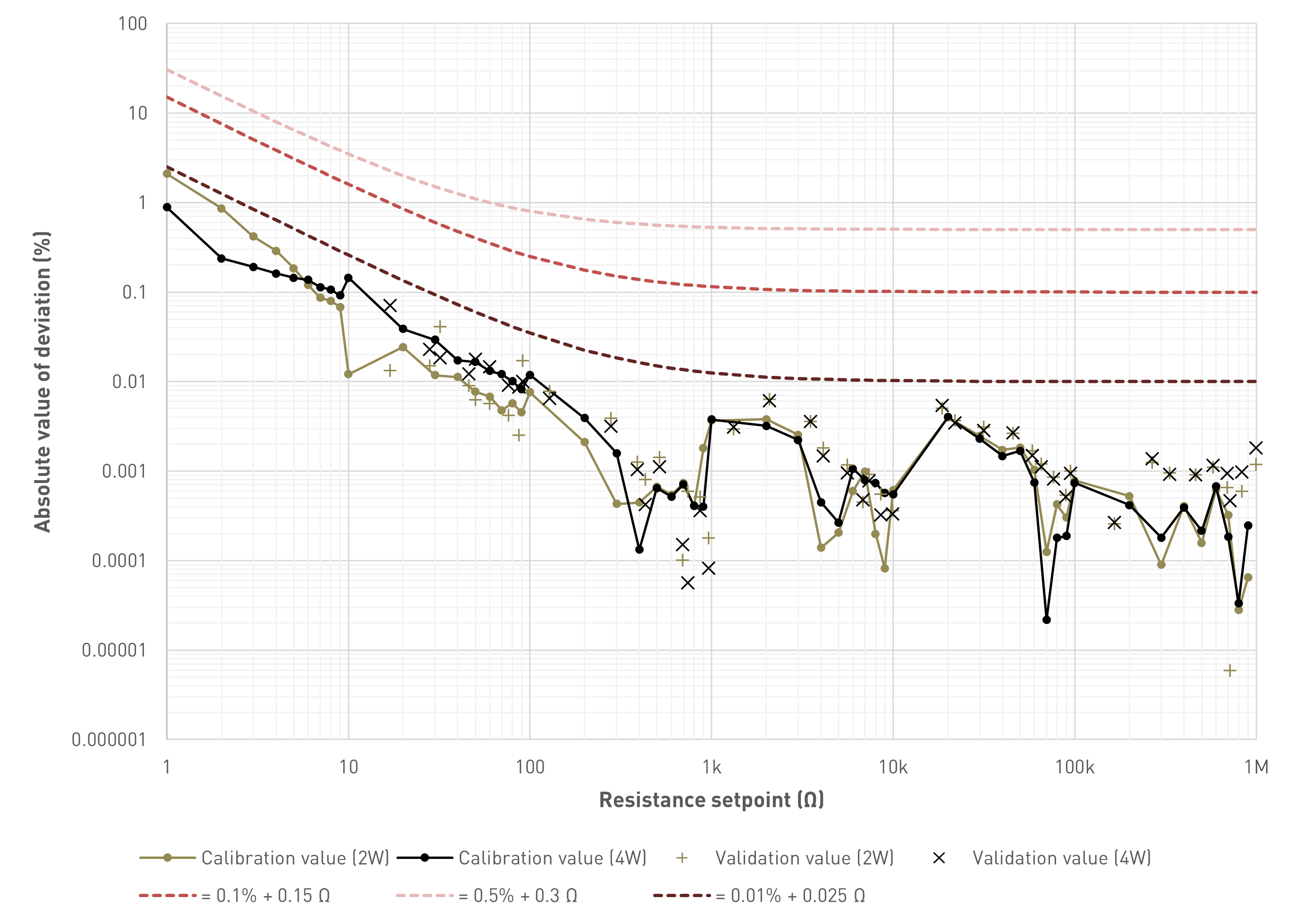
Accuracy of the resistance

The second diagram is similar to some extent, but instead of comparing the setpoint with the actual (measured) resistance, now we compare the calculated resistance (estimate based on the calibration values) with the actual (measured) resistance. This answers the question of whether we have to measure the resistance each time we select a value, or whether it’s ok to just look at the display and trust that the value displayed is the resistance at the input.

Absolute value of the deviation between the calculated resistance (estimate based on calibration values) and the value indicated by the Agilent 34401A multimeter. Connecting lines between data points for visual purposes only

Like with the accuracy, for the lowest resistance values there is some significant deviation* (worst case about 2% for two-wire and 1% for four-wire measurements at 1 Ω). However, the deviation drops really quickly. For resistance values above 10 Ω we're looking at about 0.1% (without any additive constant) deviation or less, for 100 Ω and up at a deviation of about 0.01% or less which I consider irrelevant in almost any situation this unit could be used in. In other words: In most cases the estimate is roughly one order of magnitude more accurate than the accuracy of the resistance. This leads me to the conclusion that the calculated resistance can be relied upon, with certain caveats for really low values (however, those apply for the accuracy too).

* This deviation could likely be reduced further with a software update that also stores the calibration data for the lowest decade without any compensation for the contact resistance etc. that is only required for higher decades. Shall I try it?

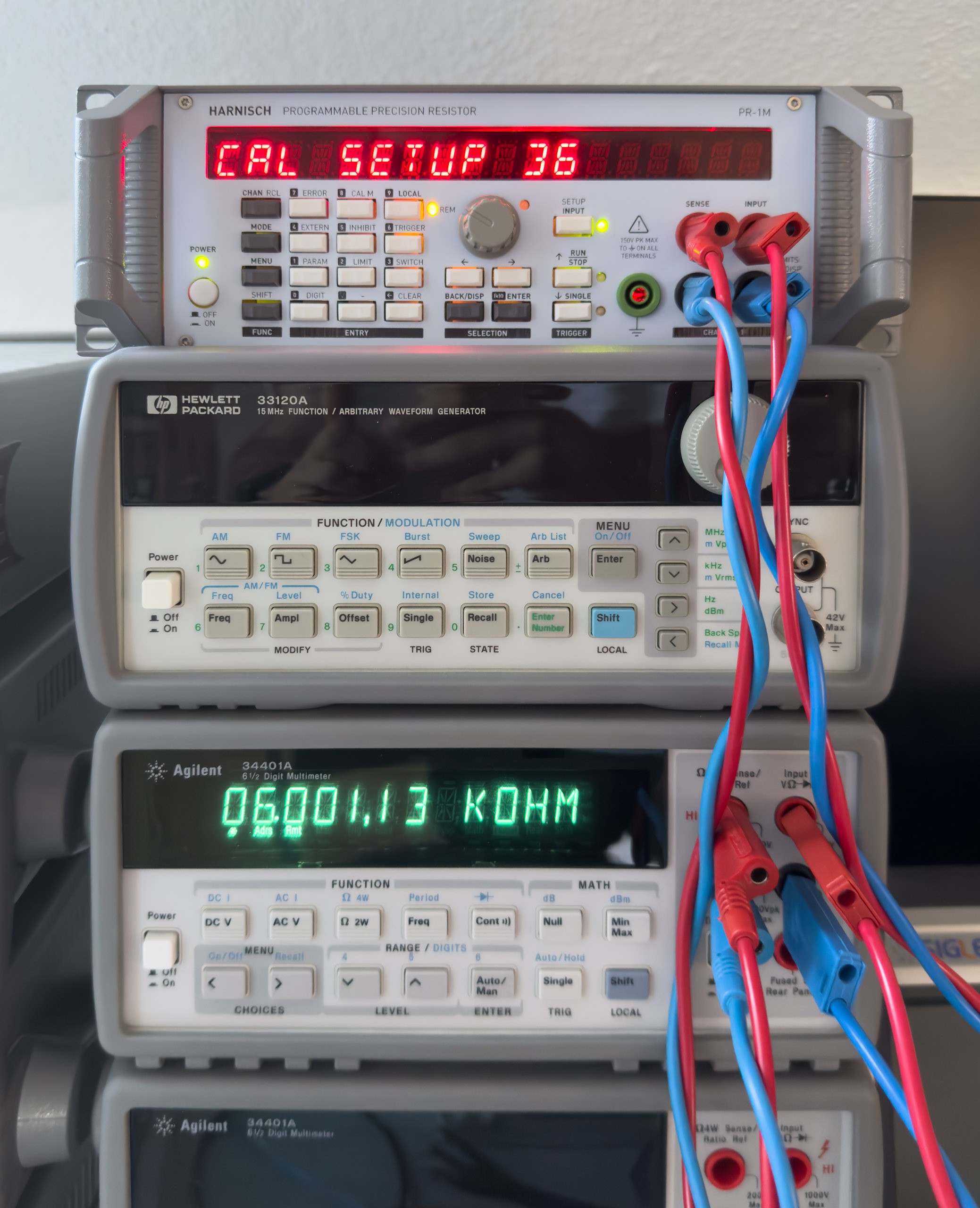
Automated adjustment/calibration setup using an Agilent 34401A multimeter.

Conclusion

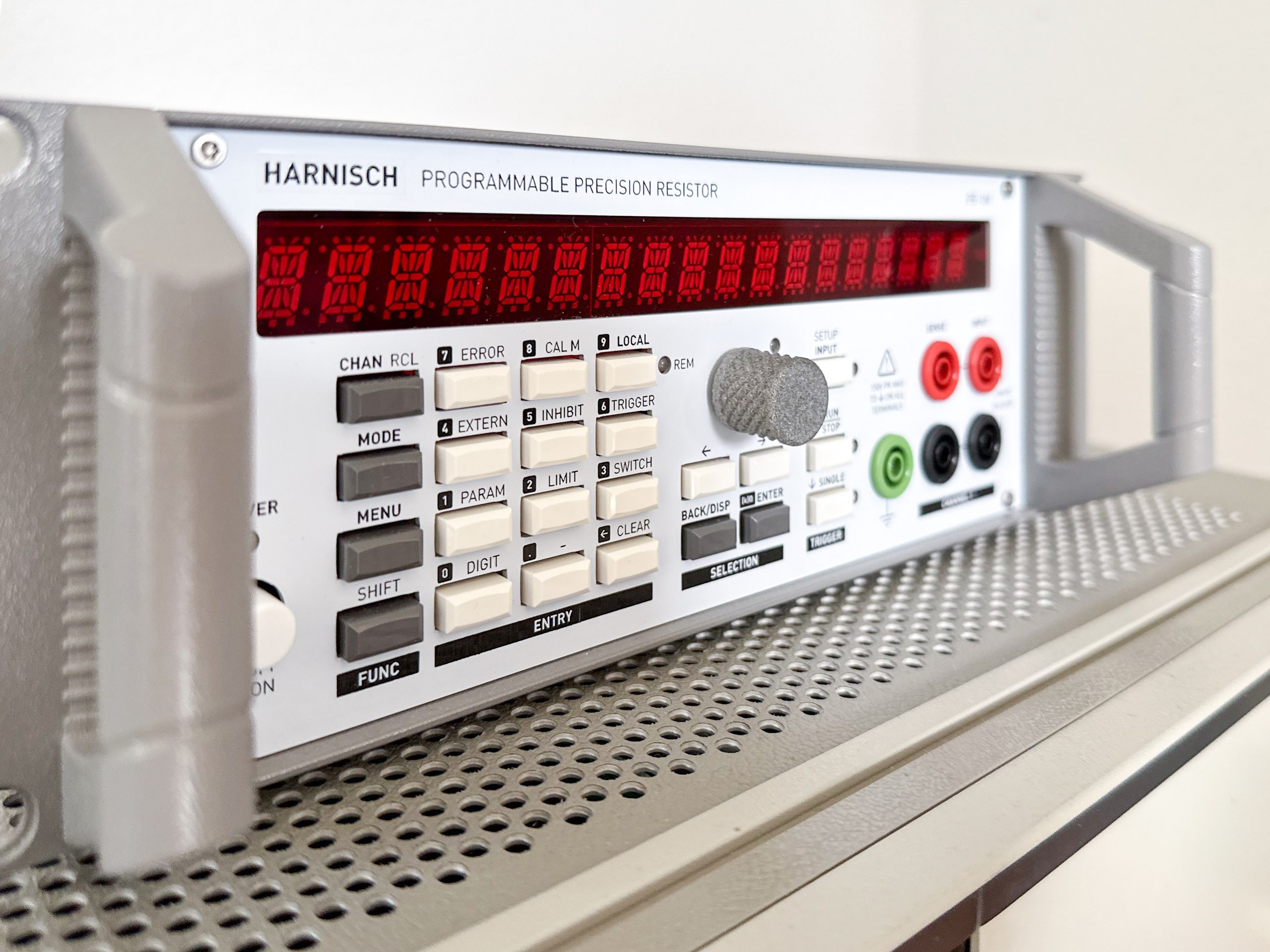
With the fairly stable resistors used and also great calibration results I think it's fair to call it a precision instrument. Hence the label Programmable Precision Resistor on the front panel. That being said: If you're looking at an accuracy in the ppm range, things like EMF and the isolation material of the binding posts matter. Those effects were not properly considered.

Also, there are some other topics that could be very interesting like temperature and long term drift (e. g. 30 days, 90 day, 1 year). I don't have a climate chamber, but re-running the automated calibration procedure in a few months would certainly be an option. How do I know which of the instruments has drifted though? And if no change can be measured, maybe both have drifted, but in opposite directions. This gets difficult really quickly :)

I went into this project with the thought that it will be a rather small one. This certainly influenced some decisions I made along the way. Now that the project had evolved into a much larger thing than initially anticipated it’s reasonable to have another look at possible optimizations, albiet the calibration results were already pretty satifactory. A small modification - seen in the following picture - can make quite a difference, so why not do it?

A green 20 kΩ resistor soldered on top of the 20 Ω resistor in order to improve accuracy for low resistance values. Note the similarities of the PCB layout and the second schematic shown below.

The contact resistance again

From the start it was clear that the relays’ contact resistances will reduce the accuracy of the programmable decade resistor, especially in the lower two decades.

To mitigate this issue I used high quality relays and paralleled their two poles. To further improve accuracy I added bypass relays for the lower three decades that bypass effectively shorted higher decades. What I did not do though: Adding footprints to improve accuracy by measuring the actual resistance and connect a matching resistor in parallel to the "main" resistors. Again, this was intentional to reduce complexity and the required board space. Also, the contact resistance is not constant, so there will always be some deviation caused by the relays. And with the topology I selected it’s not quite so easy to compensate for the contact resistances, because the contact resistance varies between odd and even resistance values. These problems are a byproduct of reducing the number of relays required.

And of course, shorted decades (nominal resistance of 0 Ω) will always have a residual resistance, bypass relays present or not. Shall we compensate for those as well to get better accuracy for the lower decades at the cost of the higher decades where the bypass relays are not available? One could argue that it would be preferable to do so, because a few milliohms do not matter for larger values.

Solutions

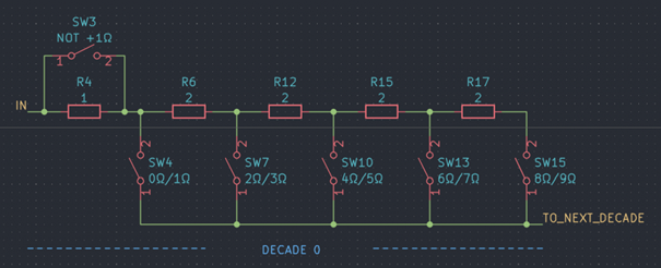
That being said, improvements can be achieved even if the result will be far from perfect even after the optimization. Let’s take a look at the schematic of the first decade:

Simplified decade resistor topology

There are two variants I’d like to discuss that improve the situation:

• Variant 1: We connect resistors in parallel with R4 and R6 respectively that reduce each resistance by about one relay’s contact resistance (as per calibration results about 25 mΩ).
• Variant 2: We only use one resistor, parallel to R6, so that the resistance is reduced by two times the contact resistance (50 mΩ)

We can clearly see that both solutions are not perfect. I prefer variant 2, because this improves the situation significantly for all resistance values greater than 1. In contrast, with variant 1 we have a large offset of about two times the contact resistance for all even values, whereas for odd values we have reduced the offset to ~0: The error varies significantly between consecutive resistance values.

But how would we calculate the resistance required for variant 2? The calculation is very simple. With R_p as the resistance of a parallel connection and R_p1 and R_p2 as the branch resistances we get:

Let's say we want to decrease R6 by 50 mΩ, then we calculate the value of the resistor R_p1 to be connected in parallel as follows:

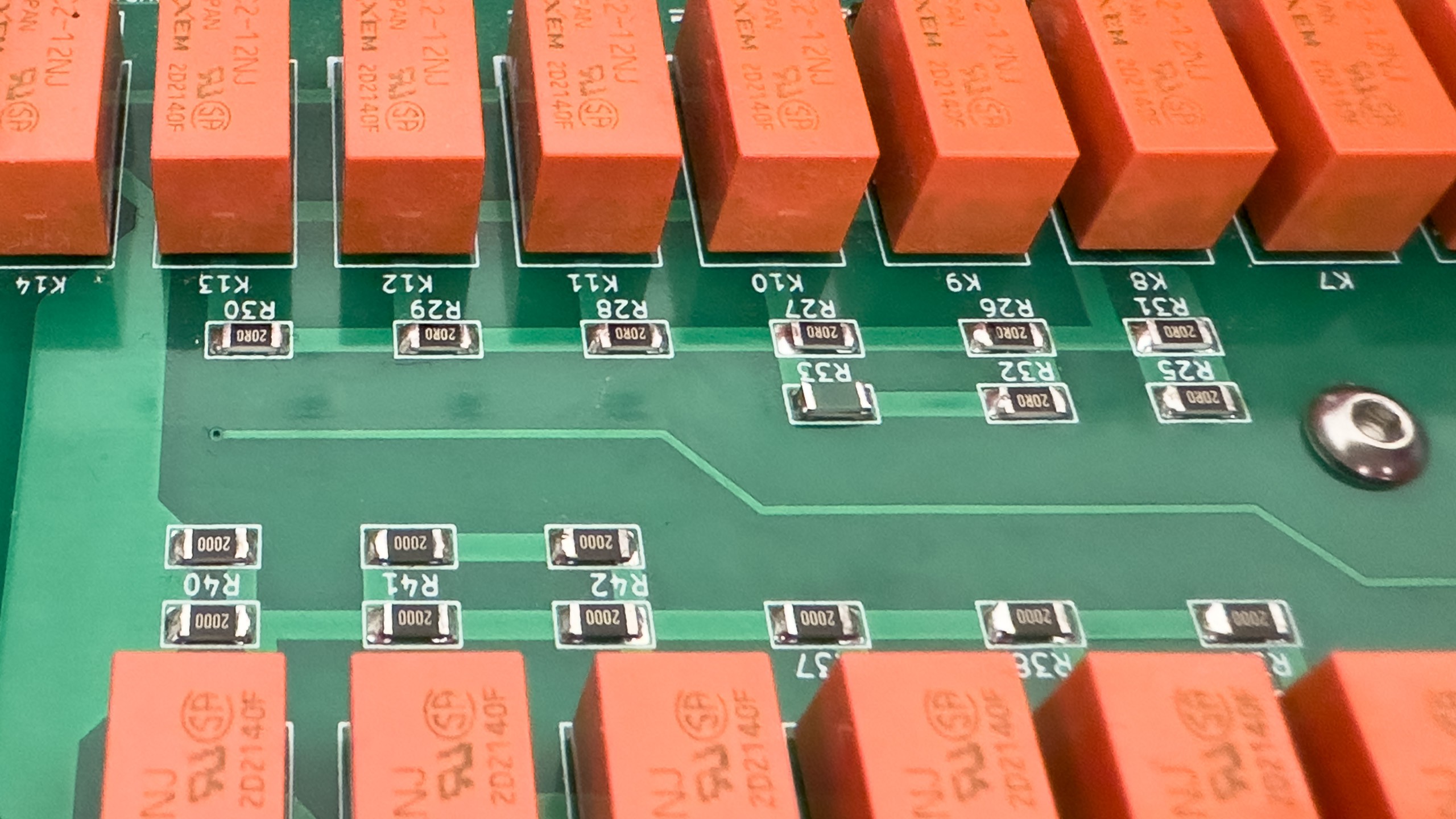
Implementation

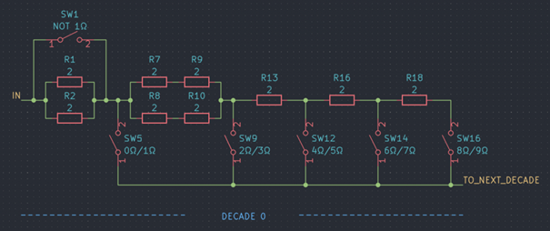
In reality, we used 4 resistors (R7 - R10) in place of R6 from the schematic above. This leaves quite some options to implement the parallel connection.

Actual topology

Every decade uses nine resistor of the same value. In order to get a bulk discount I ordered ten for each decade, so I have one left. I wonder whether I can use the tenth resistors here. Sure enough: I would simply solder the tenth 20 Ω resistor in parallel with one of the resistors R7 – R10 (doesn't matter which). This will reduce the resistance by about 46.4 mΩ. Since there is no exact value for the contact resistance anyway, this should be good enough. (By the way: The thermal coefficient of the ten times larger resistance connected in parallel isn’t all that critical – a ten times larger thermal coefficient of 100 ppm, compared to the 10 ppm of the precision resistors, shouldn’t degrade the overall performance significantly, so a 100ppm 22 Ω would do fine). And for the second decade we could simply use the 2 kΩ resistor to reduce the 20 Ω nominal resistance by about 49.6 mΩ.

And this is what I did and what can be seen in the picture above: A green 20 kΩ resistor on top of a 20 Ω resistor (second decade).

Next steps

With this modification done it's time for the final calibration.

In one of the previous logs I covered in depth, how I use the term “calibration” in the context of the programmable decade resistor and how the calibration procedure works. Now it's time for an initial test of the calibration procedure. To automate the calibration I wrote a little Python script that interfaces with the programmable resistor as well as the multimeter (Agilent 34401A) via PyVISA and SCPI commands.

Automated calibration procedure using SCPI commands

Adjustment/calibration results

The result table shows a selection of calibration points for the 4 wire mode. It has the following columns:

• Applied value: Value applied to the input for checking the calibration
• Calculated value: Estimation of the actual resistance, based on the previous “adjustment” procedure
• Ind. value: Indicated value/Measurement taken with an Agilent 34401A 6.5 digit multimeter
• Min: Minimum value according to initial accuracy goals
• Max: Maximum value according to initial accuracy goals
• Dev.: Deviation between indicated value and applied value in percent
• Dev. Calc. to Ind.: Deviation between calculated value based on the calibration constants and the indicated value

As expected, the programmable decade resistor stays well within the initial goal of << 0.5% of value + 0.3 Ω. That, however, was a pretty low bar. At the upper end, the performance is fairly impressive and showed how well the algorithm described in this post actually works. Also, the estimation of the actual resistance (that is also shown on the display) is very close to the measured value.

At the lower end, however, there is some significant deviation, mostly caused by the relay contact resistances, trace resistance and so on. 

Next steps

Before doing a proper full calibration and presenting the final results in a more user-friendly form, let's do a small hardware optimization of the design.

I was asked whether I'd be willing to share the design files. Yeah, why not... If you're interested in having a look at the different PCBs - including the panels - head over to my GitHub repository linked on the project page. Those were designed in KiCAD v7.

I generated the interactive BOM html files with an absolutely awesome KiCAD plugin written by qu1ck:

• Mainboard: HTML Preview of interactive BOM
• UI board: HTML Preview of interactive BOM
• Power Supply Board: HTML Preview of interactive BOM

I plan to release relevant parts of the code as well, same repo.

You're under no obligation to do so, but if you actually consider building this or a similar device, I would be happy to see what you did with it and maybe how you made it better.

Also, if there are aspects that you'd like more information about, please let me know.

Generally, test and measurement equipment needs a certain period of warm-up time to reach a thermal equilibrium that allows for low thermal drift. That is also true for the programmable decade resistor. I’m especially interested in the warm-up time with all relays off as well as with many relays on. I chose a value of 100 kΩ for the latter.

(For simplicity I decided against using latching relays, however that would have been a better choice performance-wise as mentioned before. Due to the additional power dissipation in the relay coils the curves will look different.)

The programmable resistor decade mainboard has two temperature sensors that can be read remotely via SCPI. To have a more complete picture I’ll also use the SCPI thermometer (previous project, https://hackaday.io/project/190792-scpi-thermometer) to sample the ambient temperature. So let’s collect some datapoints and plot a few curves.

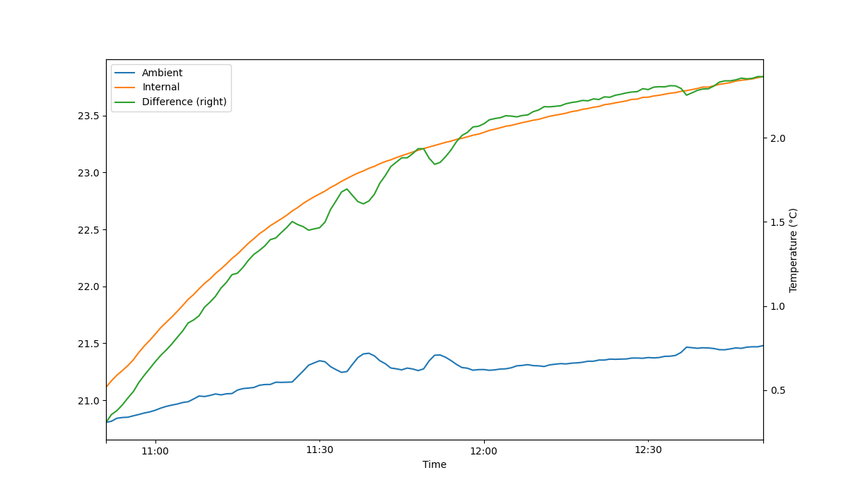
Input off

Temperature rise with all relays disabled (input off). Temperatures on the primary y-axis also in °C

Unfortunately, I had to correct a simple error in the test program so the unit was already on for a few moments, explaining parts of the gap between the internal and the ambient temperature. Also, the internal temperature sensors are not nearly as precise as the sensor used in the SCPI thermometer, so a certain deviation/offset between both sensors is expected. The temperature rise is fairly limited and it takes about one hour to see most of the temperature rise. According to the measurement it would likely take more than two hours for the unit to reach a thermal equilibrium. That being said, the steadily rising ambient temperature limits my confidence in the measurement, but hey, it's good enough.

Note: The small (positive) temperature peaks likely came from the laptop fan that switched on intermittently, although the ambient temp sensor was about 1 m away from the laptop and not (directly) in the airflow. Also, I did the measurement on a day with significant solar radiation that heated up the room. 

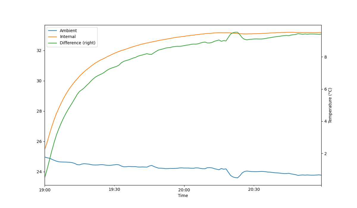
Input on

I tried to optimize the measurement protocol for the second more interestingly scenario with 100 kΩ at the input (only partially successful, I guess). Here it is:

Temperature rise with input enabled and set to 100 kΩ. Temperatures on the primary y-axis also in °C

As expected the power dissipation of the relays and the power supply, 2 W or thereabouts, increases the internal temperature significantly. Compared with the previous scenario, the final temperature increase has roughly trippled, and is now at about 8°C. After 30 min, the internal temperature rise is already at ~80% of and after one hour effectively at the final temperature. The dip in the ambient temperature was likely caused by temporarily opening a door.

Next steps

My conclusion is: Wait at least 1 hour with the input enabled and at something like 10 or 100 kΩ before going through the calibration procedure. And this is what we'll do in the next log.

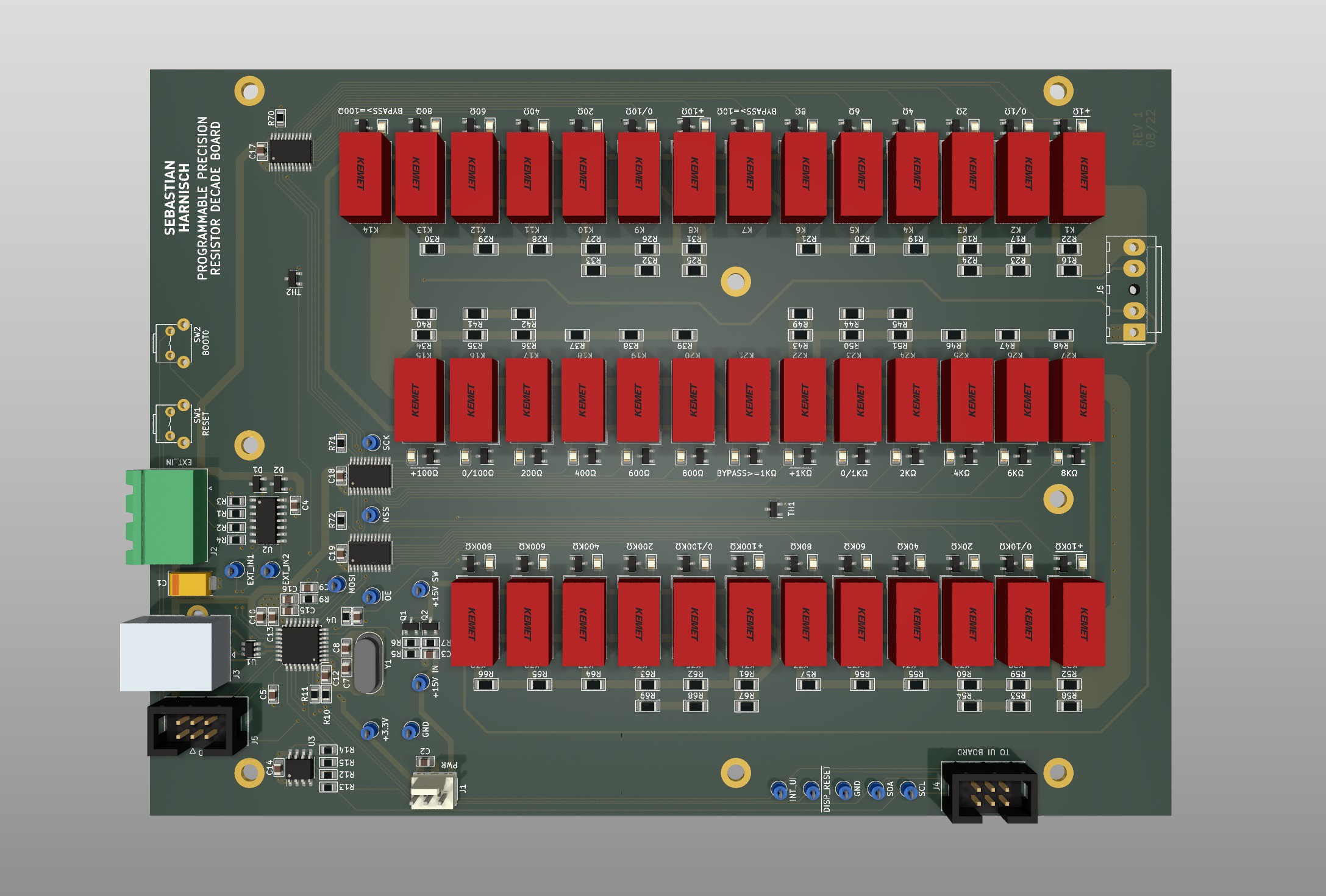
The mainboard features the main controller paired with an EEPROM, the resistor decades (precision resistors, signal relays) including two temperature sensors, relay drivers and signal conditioning for the two external digital inputs.

Rendering of the mainboard PCB generated with KiCad

Main controller

The main controller is a STM32G441KBT6 microcontroller (170MHz Cortex M4, 128kB Flash, 32kB RAM). The microcontroller features a USB 2.0 device peripheral.

The main controller contains the business logic required to control the relays and provide a user interface. It handles the processing of user user inputs, originating from either the mentioned user interface board, from SCPI messages sent over USB (virtual COM port) or from the external digital inputs.

Voltage, current and power limits are calculated based on a given resistance setpoint. Resistance setpoints are translated into switching sequences and sent to the relay drivers via SPI. Also, the main microcontroller manages all required calibration data and user settings.

An I2C-EEPROM (32kBits) is used to store different data related to the operation of the programmable resistor. Data integrity is validated with a CRC checksum. The data stored include the following:

• Calibration data (2W CAL, 4W CAL, CAL information)
• Instrument settings (e. g. Buzzer on/off)
• User settings (presets)

Relay driving circuit

To drive a total of 39 non-latching relays, three low voltage 16-bit constant current LED sink drivers are used. They essentially operate as a 48-bit shift register controlled over SPI by the main microcontroller.

Admittedly, the choice of a constant current LED driver as a relay driver is a bit odd. However, the operating conditions of the part allow for it and the part was chosen to drive the LED display on the UI Board, hence available. Care must be taken to select a constant current that is well above the minimum current to operate the relay properly.

A visual feedback for prototyping was achieved by adding a LED in series with every relay. As a side-effect the LED reduces any potential power dissipation in the constant current driver when operating a 12V relay on the +15V rail. That being said, this design might reduce the reliability of the unit: A defective LED would cause the relay to not operate. Not a big deal for my hobby applications, but if I had to build a unit for commercial use I would use a different driving circuit and not populate the LEDs. (I would use latching relays and therefore use a completely different drive circuit anyway. But that would be a discussion for another log.)

Temperature sensor

The mainboard features two KTY81-210 temperature sensors (PTC). The analog voltages of the voltage divider used are digitized with two of the 12-Bit ADC channels built into the main controller. The converted readings can be accessed through both the SCPI and the user interface. During calibration the temperature is recorded and saved to the EEPROM after completion.

External inputs

Two external, earth-referenced inputs can be used as either a simple digital input (that can be read through SCPI), a trigger input (positive, negative, either) or an inhibit signal (latching, live). Both are Schmitt-Trigger inputs and feature a resistor/diode protection circuit that allows for voltages exceeding the internal supply voltage of +3.3V.