Construction

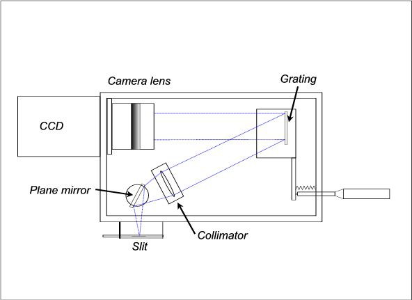
The design is significantly different to the "classical spectrograph" in that the input slit and CCD detector are at 90 degrees to each other. A schematic diagram of the basic components of can be seen here:

This next image shows the beginnings of the spectrometer showing a partially completed housing.  

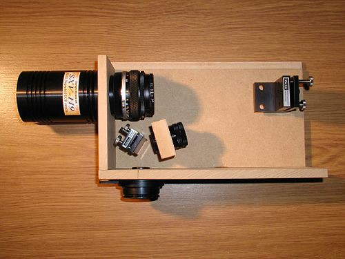
Since I do not have access to a metalworki shop but use only hand machine tools, my first choice for materials for the main body of the spectrometer was wood or wood composite (MDF). As an example, a block of MDF of dimensions 60x40x20 mm, with a 30 mm hole, serves as the support for the collimator lens and lens barrel as shown above.  Nothing could be simpler!

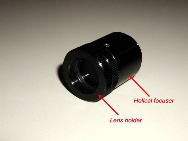
Below is an image of the collimator lens in its lens holder. The lens is an achromatic doublet with focal length of 90mm. A helical focusing tube, with a very fine thread, allows for small adjustments to be made for final collimation and is then locked in position with a small set screw. Available from Edmund Optics.

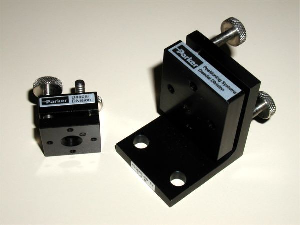
I chose to use commercially available supports for the front surface mirror and the grating mount. Since a wooden body lacks the rigidity of metal, good quality positioning mounts were selected so that more precise adjustments could be made (if needed) and any flexure compensated for. Commercial mounts like these can be obtained from companies such as Newport or Edmund Optics or Thorlabs.

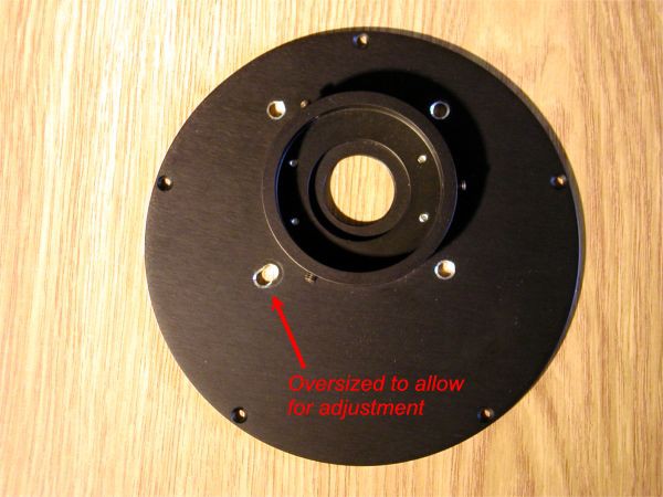
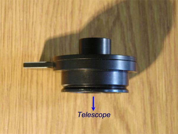
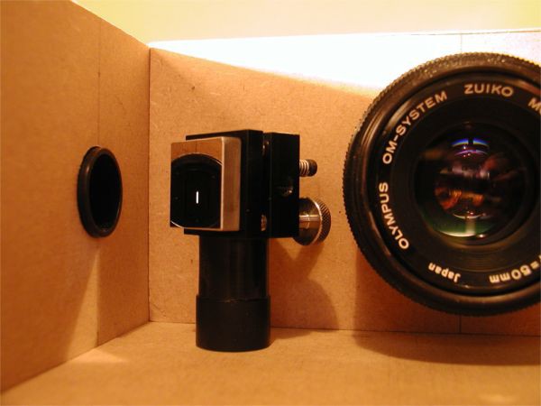
For connecting the spectrometer to the telescope, a circular plate from an old dismantled CCD camera was salvaged. Therefore never throw anything of potential future use away! The large central hole had been tapped  to receive a standard CS-mount video camera lens. This is useful for times when you may want to record the spectra of non-astronomical light sources without the telescope:

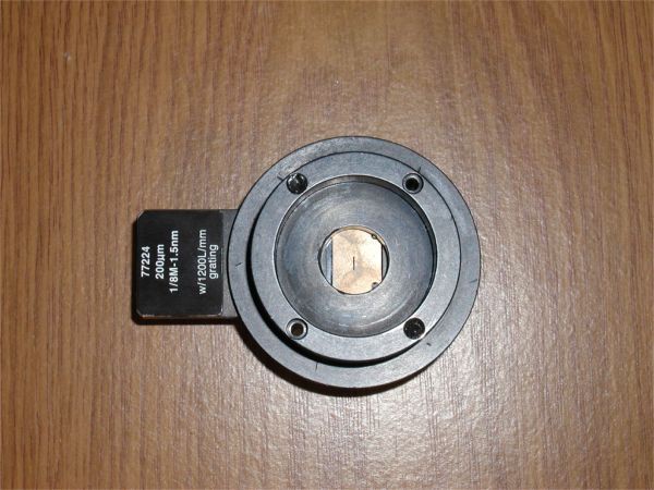
The next 2 images  are of the slit holder with one of the interchangeable slits seen inserted on the side. This holder came from an Oriel MS125 1/8 metre focal length spectrograph. The slit holder fits snugly into a hole in the side of the spectrometer. Remember that with this spectrometer design the slit and detector are at 90° to each other. Using a plane front surface mirror just after light passes through the slit does result in some light loss (the mirror’s reflectivity is about 96%) but this was considered acceptable.  The main advantage comes from the reduction in size of the whole instrument.

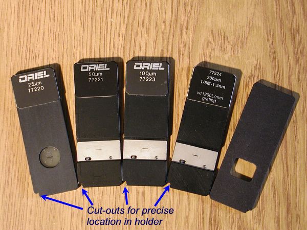
The next image is the family of 25, 50, 100 and 200 micron slits used with the spectrograph. Again, these originate from the MS125 and are available from Oriel-Newport Corp. or can be found on eBay. The “slit” on the right is simply a square hole that can be used for wide slit or slitless spectroscopy. The small square cut-out at the bottom right-hand corner of each slit enables the aperture to be positioned precisely and reproducibly at the centre of the slit holder (previous photos).

This next picture is a preliminary alignment test. I am observing from the position of the diffraction grating to check for correct plane mirror orientation. Fine adjustments with the collimator's helical focusing ring produced a sharp clear image of the slit which is now collimated. Thus light rays focused on the slit will be parallel when incident on the grating.

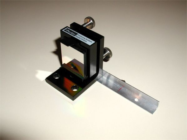
The following image shows the grating with a “rotation arm” bolted to the grating mount. This is simply a length of 10 mm angled aluminium strip and is used to provide controlled rotation of the grating when coupled to a micrometer adjustment screw. Just about visible in this picture, behind the angle bracket at the red line marking, is a knurled nut that has been glued to the arm at a precise position. Seated in the nut will be a small hardened steel ball which will maintain contact with a micrometer screw via a suitable spring attached to the arm and the rear wall of the spectrograph.

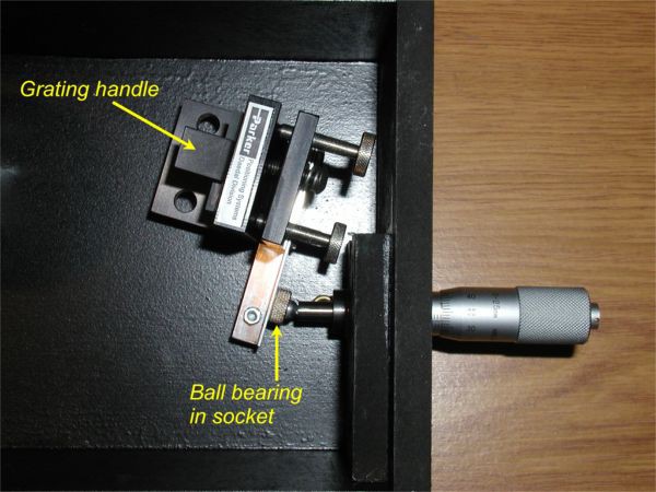
The mechanism used to provide rotation of the grating, and to allow different wavelength ranges to be detected by the CCD camera, is shown in the next two images. A micrometer screw pushes against a hardened steel ball in a small socket. Firm (but not too firm!) contact between the micrometer and ball is maintained with a tensioning spring of the right force constant that I retrieved from an old ink-jet printer. When rotated, the grating arm moves through an arc of radius about 39mm.

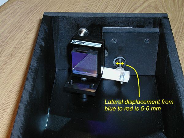
I am using a 1800 lpm grating with this spectrograph, and I want to have access to the whole visible spectrum from about 380 nm to the near IR at about 900 nm. When turned throughout the full wavelength range, this angular rotation corresponds to a lateral displacement of just over 6 mm between the point of contact of micrometer screw and the steel ball.

Since the diameter of the micrometer screw is exactly 6.35 mm, some careful experimentation is necessary to ensure the extreme wavelength limits in the violet and the near IR are still accessible without the screw and ball losing contact. This procedure was done by trial and error.

The micrometer screw chosen must also have enough linear displacement to cover this wavelength region. The model I found from a local supplier has a total linear translation of 25mm which is acceptable for a 1,800 lpm grating. The total distance covered from blue to near IR is about 21mm.

Finally, two views of the completed spectrograph are given here in its final version. The original Olympus f/1.8 lens has now been replaced by a Pentax f/1.4 50mm lens and the camera and lens brought as close as possible to the grating without cutting off the 18mm f/5 parallel beam from the collimator lens. An earlier experimental configuration had the CCD camera and lens about 60mm further away from the grating. However, this suffered from severe vignetting at the camera lens, causing a loss in signal intensity at the edges of the CCD sensor.

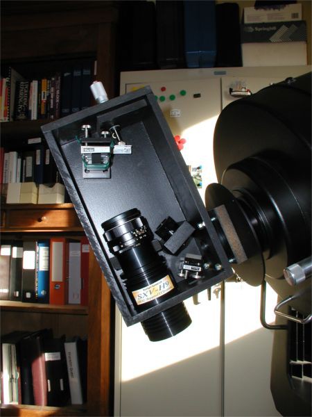
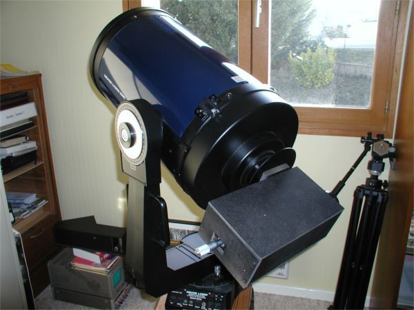
The spectrograph measures 27cm x 15cm x 10cm. Compared to my previous attempt as mentioned in the intro, it is a significantly more compact unit and weighs much less, even with the CCD camera and large telescope adapter needed to hold it in place. The theoretical resolving power R = 2000 with the 1800 lpm grating.

Evaluation and Testing

The Solar Spectrum

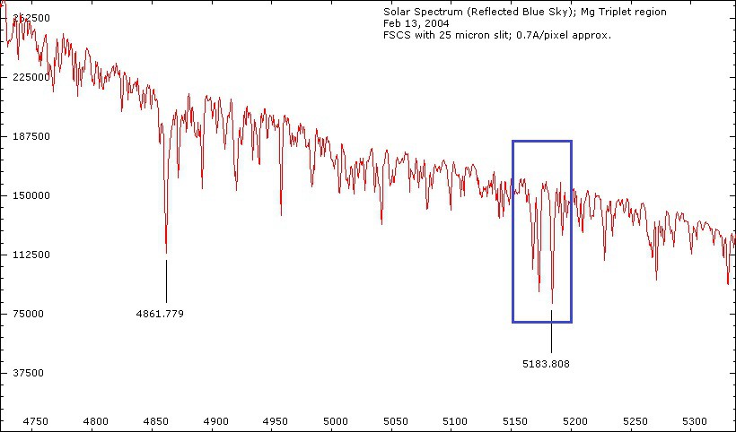
To test this improved version of the spectrograph the solar spectrum (from reflected blue sky) was recorded. Several specific regions of the visible solar spectrum are presented below. This was mainly to check the resolving power of the spectrograph and to test its sensitivity at the extreme ends of its range. None of the spectra have been calibrated in intensity (vertical axis in the line profiles). I was more interested in verifying the practical resolution of the instrument at this stage, which from the results below appears to be close to the theoretical value.

A group of solar absorption lines known as the Magnesium Triplet around 5180 Angstrom units (Å) is a common test of the practical resolving power of any spectrograph. This region falls near to the maximum sensitivity (65% QE) of many CCD detectors. The sensor in this detector is a Sony ICX285AL sensor and the camera model is a Starlight Xpress SXVH-9.

An exposure of only 1 second, while pointing the spectrograph at sunlight reflected from a bright blue sky, was enough to record the spectrum given below. At these short exposures the subtraction of a dark frame is not necessary. The dark current of the Sony sensor used is exceedingly low. In fact, the manufacturers of the camera do not recommend dark frame subtraction for exposures less than 10 minutes. Subtracting a dark frame from the raw image can do more harm than good since the statistical noise of the dark frame may exceed the pattern noise from hot pixels and consequently add to the result of the dark subtraction.

Any “hot” pixels, which are principally caused by cosmic rays passing through the sensor chip, can simply be eliminated using image processing software. The images below were pre-processed using either IRIS or ImagePro Plus software. Since perfect alignment of the grating grooves and vertical pixel columns of the CCD chip is never or rarely achieved the first time, controlled rotation of the image is usually required prior to binning to give the spectral profile.

The following two images show the Balmer H-alpha region in the Sun's absorption spectrum, first as the raw image, and then as the spectral profile. 

Atmospheric O2 absorption lines around 670nm are clearly evident. The raw spectrum image exhibits some slight curvature (a very common effect, especially for home-made spectrographs) which has not been corrected for. This has probably degraded the resolution slightly during the binning process to obtain the spectral line profile. Any corrections for line curvature would slightly increase the resolving power.

This next spectrum is a closeup of one of the several atmospheric H2O absorption bands in the solar spectrum, this one around 670 nm. Note that the x-axis here is in pixel number and not wavelength!

And finally, as an earthbound example, are two emission spectra of the famous Swan bands of the dicarbon molecule (C2) observed in hydrocarbon flames. These were obtained by simply pointing the slit of the spectrograph at a propane-butane CampingGaz stove:

For More Information...

More spectra obtained with this home-built spectrograph, together with much more information on this and other spectrometer designs, can be found on my Blog at Steve's Open Lab