This is a proof of concept to show how sensory and state information can be represented using a population of modified Izhikevich neurons. The examples here read an angle from the environment; this can be considered the angle of a joint on a limb. In biological systems this angle would be determined from the integration of various sensors but in a synthetic system can be determined by a potentiometer or encoder. Each neuron in a population code corresponds to a specific value in a state space, with the firing rate of each neuron determined by proximity to that specific value. In these examples the proximity is given by a Gaussian function where the peak is centered on the threshold of the neuron, and the coefficient and standard deviation are arbitrary. As the firing rate of each neuron is a function of its input current, this Gaussian function provides a bias current per neuron.

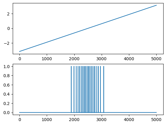
Here is an example with one neuron that senses an angle of zero. The angle is given in radians in the top plot, while the bottom plot shows the firing sequence.

i = 0
def demo_classiexcitable():
    time = 5000
    count = 1
    tau = 1.0
    t = np.arange(0.0, time, tau)
    v = np.zeros((t.size, count))
    u = np.zeros((t.size, count))
    fired = np.zeros((t.size, count))
    signal = np.arange(-np.pi, np.pi, step=tau*2*np.pi/time)
    global i
    def trace(neurons, synapses):
        fired[i] = neurons[0].fired
    def read_input():
        return signal[i]
    cells = neuron.PopCode(count, threshold=np.array([0.0]), 
                    read_input=read_input,
                    calculate_bias=lambda angle, angle0: 30.0 * np.exp(-((angle-angle0)**2) / (2.0 ** 2)))
    s = sim.Sim(tau, [cells], [], trace)
    for i in range(t.size):
        s.update()
    fig, axs = plt.subplots(2)
    axs[0].plot(t, signal)
    axs[1].plot(t, fired[:,0])
    plt.show()

demo_classiexcitable()

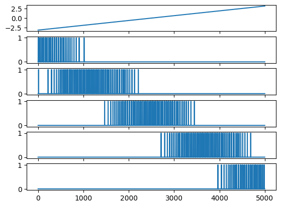
This expands this example to five neurons, with overlapping firing patterns. The limits of rotation do not wrap the whole way around the circle.

i = 0
def demo_classiexcitable5():
    time = 5000
    count = 5
    tau = 1.0
    t = np.arange(0.0, time, tau)
    v = np.zeros((t.size, count))
    u = np.zeros((t.size, count))
    fired = np.zeros((t.size, count))
    signal = np.arange(-np.pi, np.pi, step=tau*2*np.pi/time)
    global i
    def trace(neurons, synapses):
        fired[i] = neurons[0].fired
    def read_input():
        return signal[i]
    cells = neuron.PopCode(count, threshold=np.linspace(-np.pi, np.pi, count), 
                    read_input=read_input,
                    calculate_bias=lambda angle, angle0: 40.0 * np.exp(-((angle-angle0)**2) / (2.0 ** 2)))
    s = sim.Sim(tau, [cells], [], trace)
    for i in range(t.size):
        s.update()
    fig, axs = plt.subplots(count + 1)
    axs[0].plot(t, signal)
    for j in range(count):
        axs[1+j].plot(t, fired[:,j])
    plt.show()

demo_classiexcitable5()

This example is slightly different. Here, the angle and threshold of each neuron is determined by a unit vector. There are seven neurons evenly spaced around a continuous circle. This behaves more like a compass.

i = 0
def demo_classiexcitable7vector():
    time = 5000
    count = 7
    tau = 1.0
    t = np.arange(0.0, time, tau)
    v = np.zeros((t.size, count))
    u = np.zeros((t.size, count))
    fired = np.zeros((t.size, count))
    rads = np.arange(0.0, 2.0 * np.pi, step=tau*2*np.pi/time)
    vec = np.array([np.sin(rads), np.cos(rads)])

    threshold_rads = np.arange(0.0, 2.0 * np.pi, 2*np.pi/count)
    threshold_vec = np.array([np.sin(threshold_rads), np.cos(threshold_rads)])
    global i
    def trace(neurons, synapses):
        fired[i] = neurons[0].fired
    def read_input():
        return vec[:, i]
    cells = neuron.PopCode(count, threshold=threshold_vec, 
                    read_input=read_input,
                    calculate_bias=lambda v, v0: 5.0 * np.exp(np.arccos(np.clip((v/np.linalg.norm(v)).dot(v0), -1.0, 1.0))**2 / (2.0 ** 2)))
    s = sim.Sim(tau, [cells], [], trace)
    for i in range(t.size):
        s.update()
    fig, axs = plt.subplots(count + 1)
    axs[0].plot(t, vec[0])
    axs[0].plot(t, vec[1])
    for j in range(count):
        axs[1+j].plot(t, fired[:,j])
    plt.show()

demo_classiexcitable7vector()

Population Code and Rate Code

Discussions

Population Code and Rate Code

Discussions

Become a Hackaday.io Member