The making of this map can be split into a few sections: making a 2D map, making the 3D models, electronics and software and final assembly. Here I provide some details about each of these steps.

Making the Digital Map

In the past I have briefly worked with maps so I am familiar enough with some GIS tools to pull and combine data from various sources. The first step in this project was the map’s data needed to display the trains. The absolute must haves were:

1. Manhattan coastline
2. Subway routes
3. Subway stations

I also wanted to show streets, but this was not strictly necessary.

The coastline of manhattan I was able to pull from OSM (Open Street Map) with a very simple Overpass query: 

[out:json][timeout:25];
(
  way["natural"="coastline"](40.6839,-74.0479,40.8820,-73.9070);
);
out body;
>;
out skel qt;

The subway stations were also easily queried with Overpass:

[out:xml] [timeout:25];
 {{geocodeArea:manhattan}} -> .area_0;
(
    node["railway"="station"](area.area_0);
);
(._;>;);
out body;

 
The subway routes were trickier to get because I could also use OSM, but this approach had several disadvantages:

• The lines of the routes usually follow the train tracks underground which means they have some subtle curves that I would have to clean up later.
• The data has a line for each subway track, so one for each: northbound, southbound, local and express. I only needed one per color
• The data also includes the platform footprints, something I also don’t need

I found that New York City has an open data website with a lot of different sources. One of them was a subway line centerlines, exactly what I needed. Unfortunately it is no longer available in their website.

I combined all these sources in a QGIS project and exported a DXF file so I could clean up and edit the data for 3D printing. I used the ESPG:3857 Pseudo-Mercator projection. No real reason, it was the default and it looked alright so I kept it.

Real Data to Usable Data

I imported all the map data into Illustrator for cleanup. This was by far the most time consuming part of this project, in part because I needed to do a lot of tweaking and in part because of my inexperience with Illustrator. The map data is highly accurate but it also means it’s impractical for 3D printing: very thin lines represent subway lines and streets, stations are just points (no area), overlapping stations, overlapping subway lines and many other small issues.

To make the map 3D printable I did the following:

• Removed all coastline data that wasn’t part of Manhattan
• Removed coastline features that were too small to be 3D printed correctly
• Made all streets and subway lines thicker lines, then outlined them to turn them into polygons
• Added two circles per stations and move them around so they would be close to the original location but without overlapping
• Wrote a custom Illustrator script to remove all polygons that were too small to 3D print
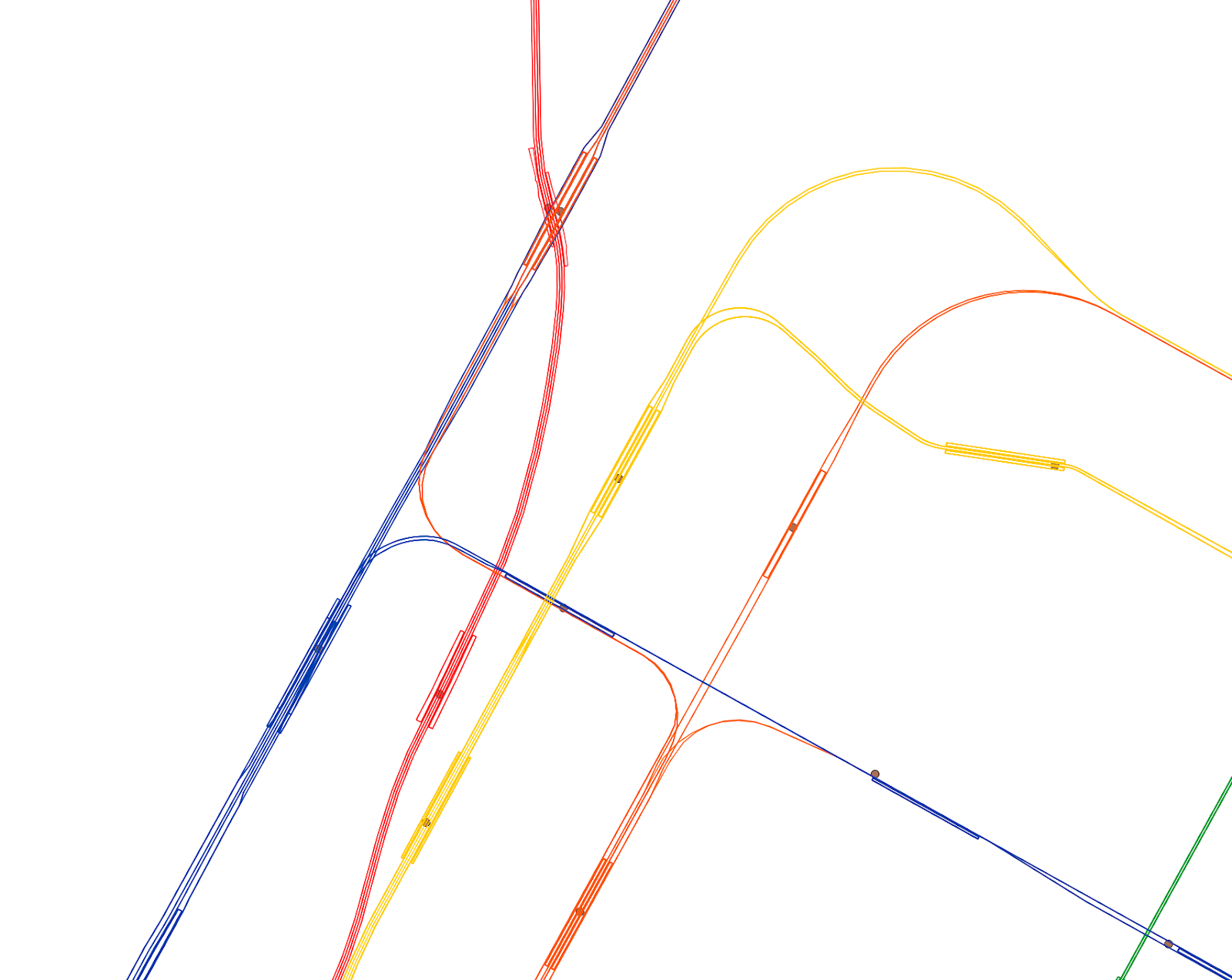
• Played around with the position of subway lines so they would be close to their original location but without overlapping

This sounds simple but it took many, many hours of very fiddly and manual labor. This was an iterative process where I would make changes to the 2D map, then export the map as an SVG, create a 3D model and either slice it or even print part of it to see how it would look.

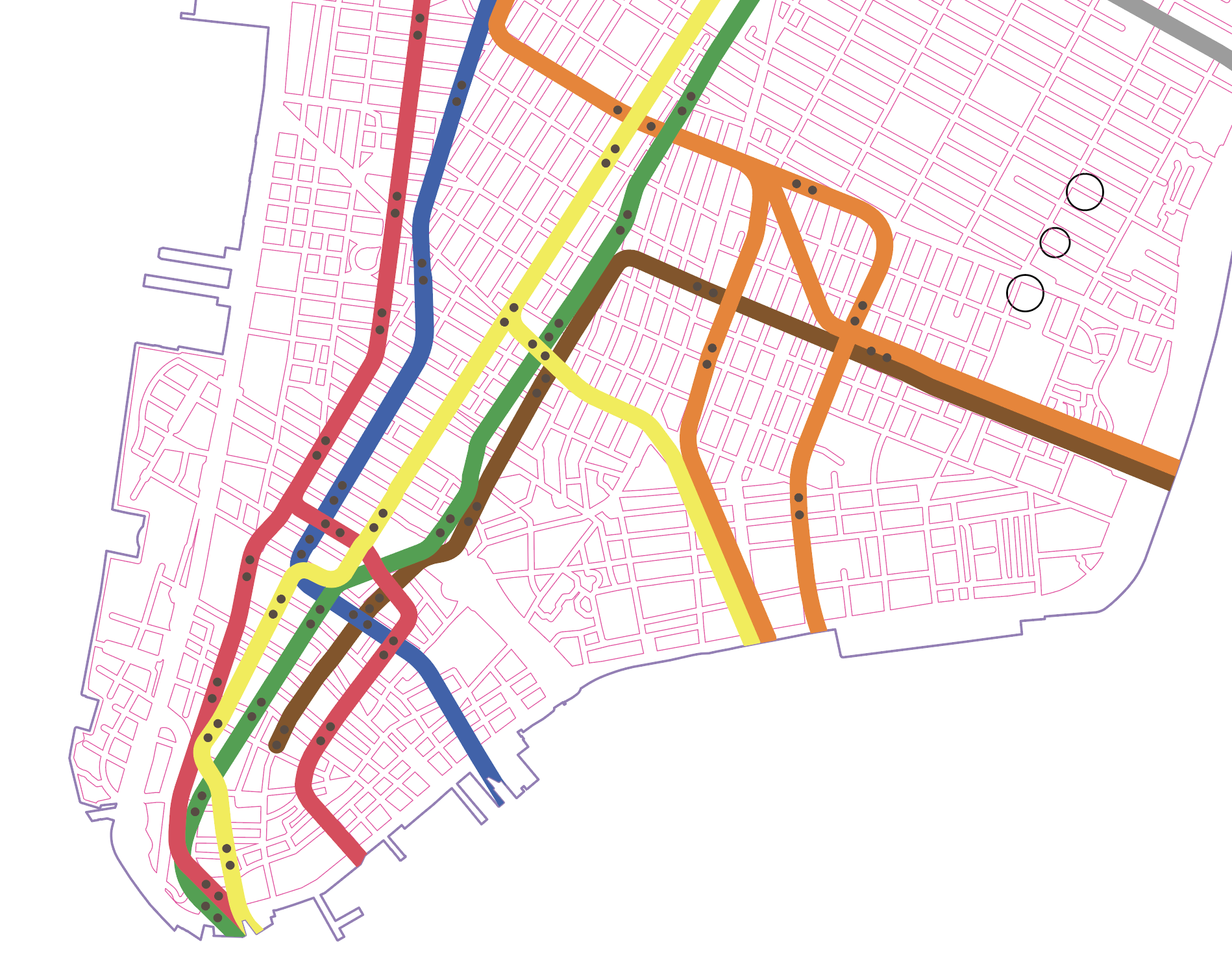
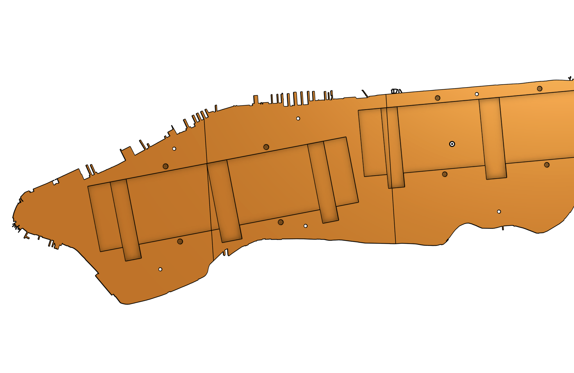
In the end, the Illustrator map also had additional layers that I would use for features in the 3D model, like the 3 black circles in the image above which represent the location of posts and threaded inserts to attach the base of the completed map to the top.

Making the 3D Models

Polygon Cleanup

I tried creating the map with OnShape and Fusion 360, both of which failed, either by slowing down to a crawl or crashing due to the number of polygons. Even the island alone was enough to make both of these struggle, the buildings/streets were a non-starter.

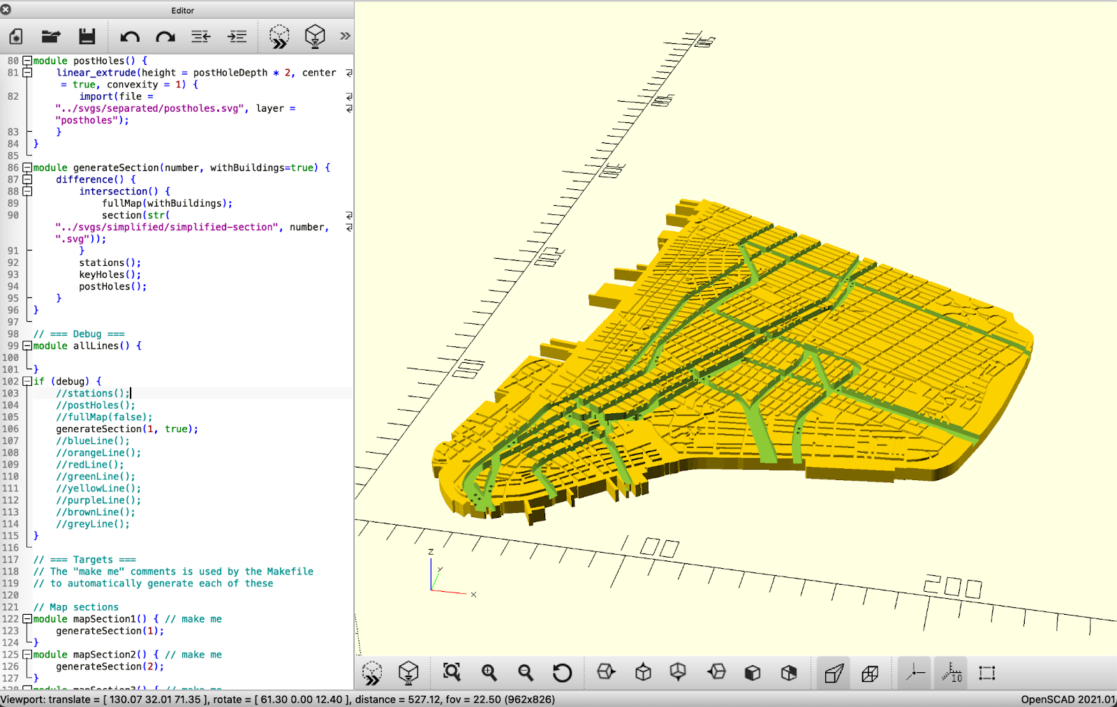
I decided to use OpenSCAD which I had never used, but it turned out to be perfect for this application. The only problem was that some of the polygons in the exported SVG from Illustrator were invalid because they had a self-intersection. OpenSCAD rightfully refused to generate a 3D model with those errors. Finding and cleaning these by hand was a daunting task which I really didn’t want to do. After a few hours of struggle and failed attempts at fixing this, I remembered the absolutely fantastic command line tool vpype. It’s normally used to simplify and clean up SVGs meant for pen plotting, but I used it to clean up all my polygons:

vpype forfile "svgs/separated/*.svg" read "%_path%" linemerge linesort reloop linesimplify filter --min-length 0.5mm write "svgs/simplified/simplified-%basename(_path)%" end

This basically turned each path in the SVG into polygons, simplified the lines and removed unnecessary vertices.

Top Map

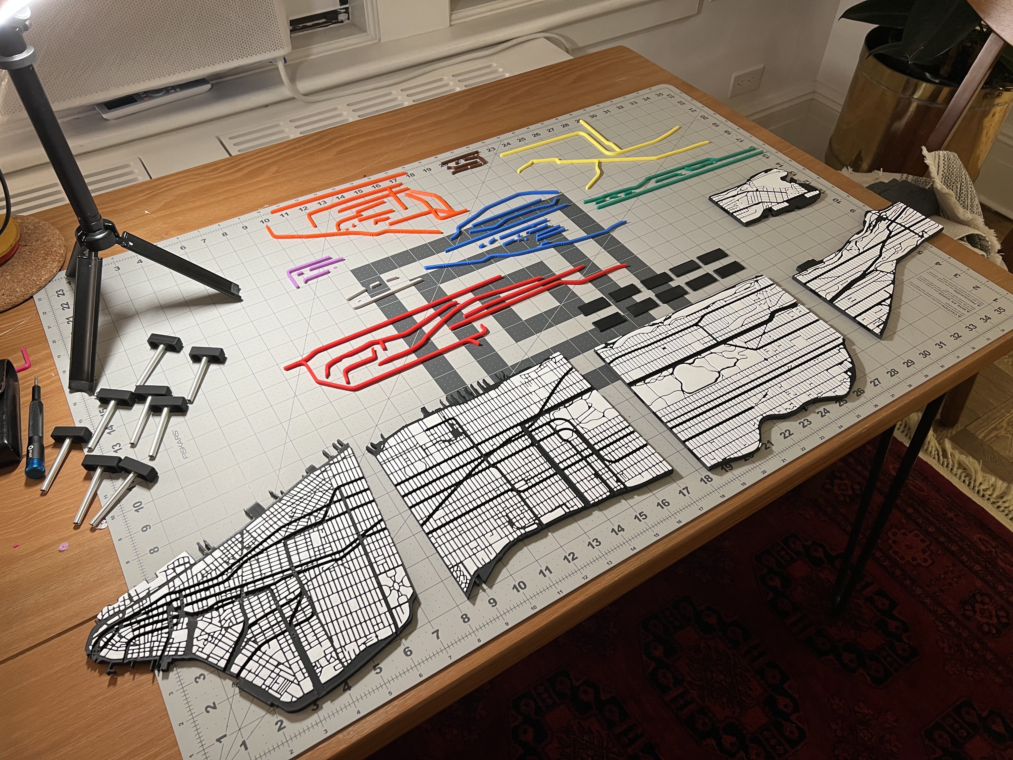
The top map is the one that actually shows buildings/streets, subway lines etc. Each layer in the original SVG was separated into its own SVG file and then cleaned up with the command above. I then imported each of these into OpenSCAD to create each STL needed for the project. I made a total of 14 STLs with OpenSCAD:

• 5 sections of the map of Manhattan
• 8 subway lines, one per color
• 1 with rectangular keys to align the sections of the island

The sections of Manhattan took a long time to generate, so I would leave my computer working overnight. I never calculated how long they took, but probably around 2 hours in total.

Bottom Map

The bottom map is the one that houses the electronics, LED matrices and fiber optics. This one was simple enough to be made in Onshape but also I made it before the top one. I would have done all in OpenSCAD otherwise. I also made a few other parts here, like a lid with holes to put on top of the LED matrices to attach the optic fiber or adapters so I could attach aluminum posts to the top and bottom layers.

Electronics

The electronics of this project are very simple. I used two WS2812B 8x32 LED matrices from Amazon daisy chained together, a Raspberry Pi 4 to control them and an external power supply. The Raspberry Pi runs Raspbian.

Writing the Software

I wanted to learn Go around the time I started this project so I decided to write all the software in Go. The software has two major components: the data fetching and the LED control.

The live location data comes from the MTA’s real time feed APIs which are free and open. There are 6 different URLs needed for this map because feeds are split by line groups. The API responds with a giant protobuf containing a lot of transit data which then needs to be parsed to get the train locations. Fortunately the protobuf definition is part of the GTFS (General Transit Feed Specification) and there are plenty of libraries for it. I used Mobility Data’s GTFS realtime bindings for Go here.

While parsing the protos were simple, understanding them was much more complex. My current understanding is the following:

• There are 2 types of entities: vehicle and trip_update
• Vehicles will show "current_status: STOPPED_AT" and a stop ID of where it's stopped
• If there is no current_status for a vehicle, then I assumed it was in transit to the stop ID
• Vehicles also have a route ID that can be used to figure out the type of train (A, C, E, 1, 2, 3, etc)
• The entity's ID can be used to correlate the vehicle to the trip_update.
• The stop ID can be used to determine the direction of the train, because it ends in N or S for north and southbound. In New York City’s transit system, there are only 2 directions, North and South, even if geographically a train may be moving East-West.

Every 30 seconds the software polls the GTFS feeds, finds all tracked trains based on lines (discarding the Grand Central shuttle for example) and determines if they are in transit or stopped. It then updates the LED matrix with the current data.

LEDs are controlled with the ledctl library. A goroutine executes on a timer every 10 milliseconds, it clears the LEDs and then sets the ones that should be set based on a buffer. It’s fairly rudimentary, but it works.

I also had to write a few tools needed to accessible, calibrate and configure the map. These are a tool for color testing so I could find the right color for each line and a tool to map a pair of LEDs to a real life station. The alternative was to pre assign LEDs to stations but that would require the optic fiber to be threaded to one exact location on the LED matrix which is far harder than just going over the map once and map light indices to a station ID.

Manufacture and Assembly

I printed each map section in my Bambulab X1C. I don’t have an AMS so I added a pause after the last layer before the buildings start, then swapped the black filament for white and continued the print. This worked perfectly well.

The subway lines were also fairly simple to print except I needed to manually trim some of the lines because they were too long. I did it directly in the slicer. I didn’t have PLA of all the colors I needed and since I only needed a small amount of each I bought a couple of color sample packs from Amazon which included all the colors I needed. The only problem was that I only had about 3 m (10 ft) of filament, so I needed to change filaments often.

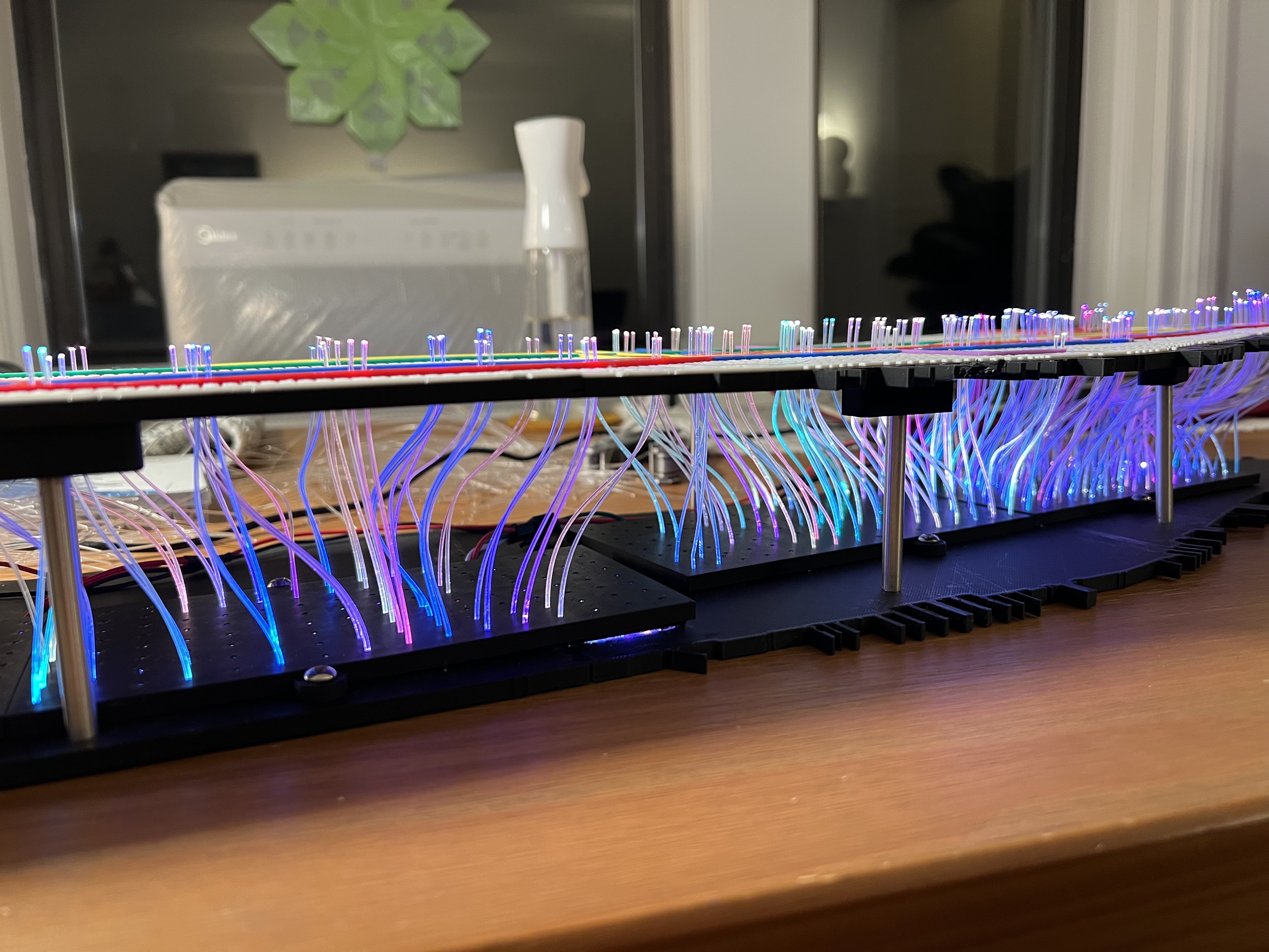
After all the parts were printed I assembled the bottom and top maps. I attached the lines to the top map with double sided tape which worked surprisingly well. Then I spent a few hours threading 1 mm diameter optical fiber through each station hole and into the LED matrix. I had to insert a metal wire first to clean up the hole, then I could slide the fiber in.

These are all the 3D printed pieces of the top before assembly and the posts are visible on the left:

Here is part of the threading process. Each strand needed to be longer than necessary during this step, otherwise they tended to slip out and rethreading them was painful. At the end I lowered the top map onto the bottom one little by little while adjusting the strands, then I trimmed them all flush with the top.

Here is a side view of the fibers right before trimming, one of the few things I knew I wanted out of this project was to be able to see the fibers from the side. At this point each LED pair is on with a random color

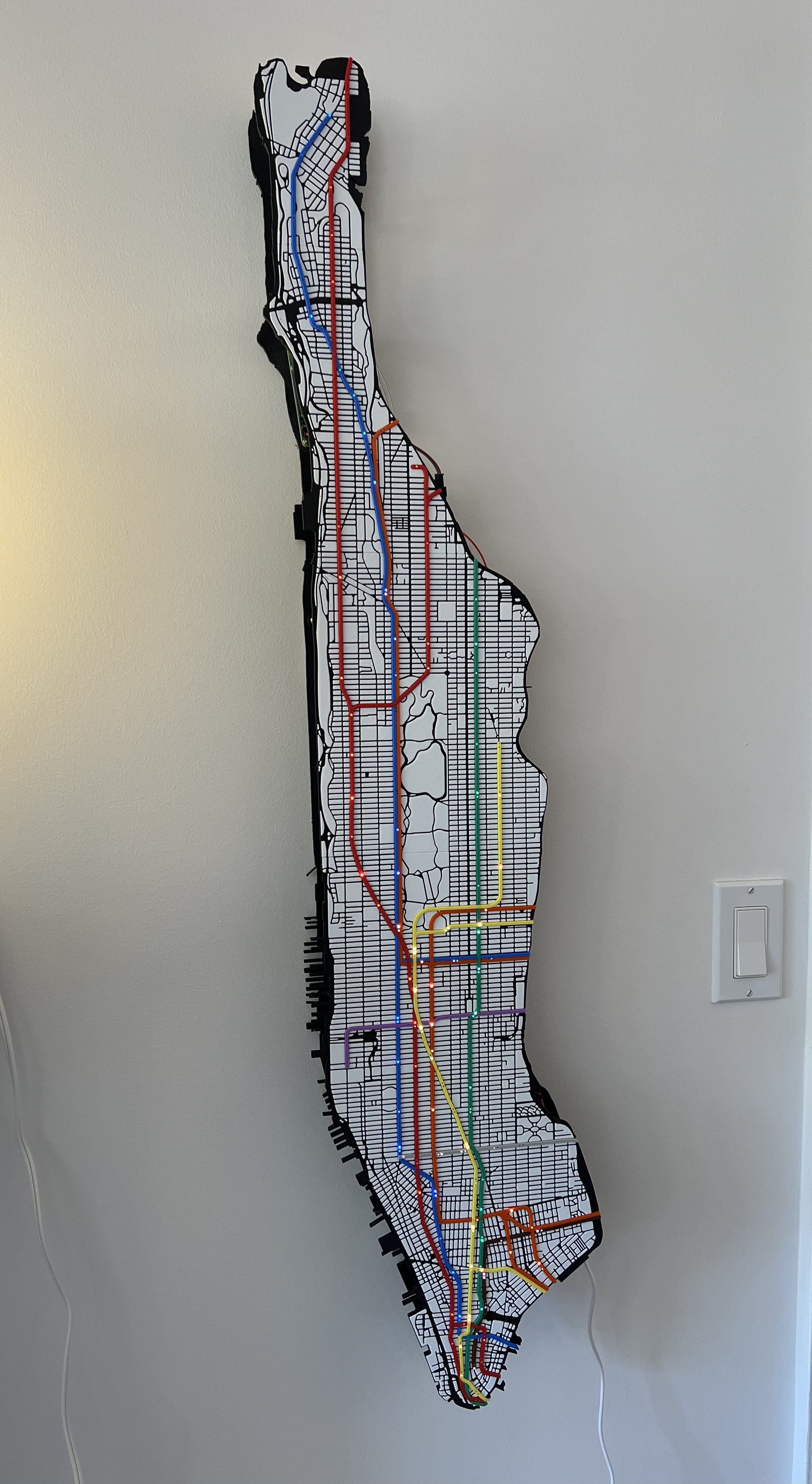
And here is the finished piece from the front: