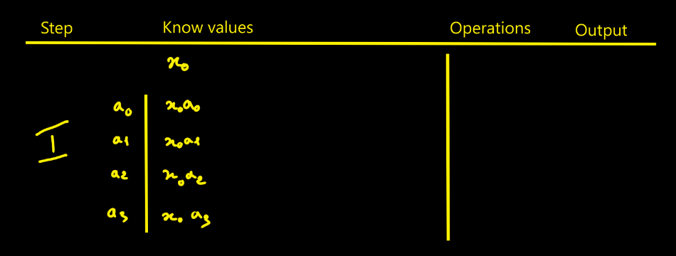
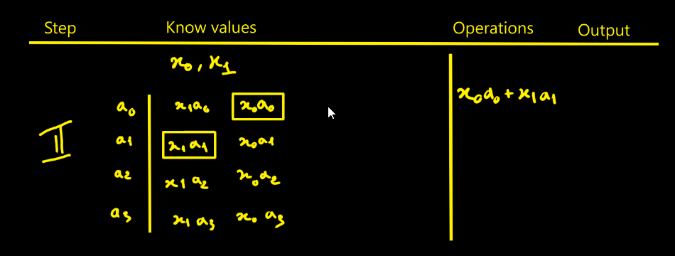
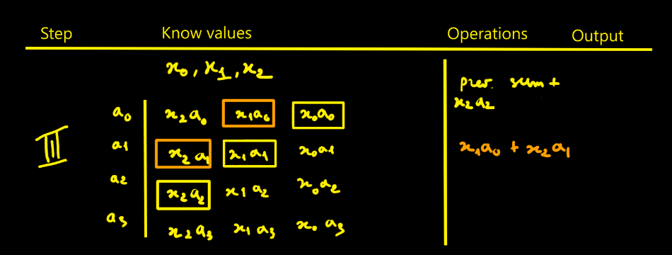
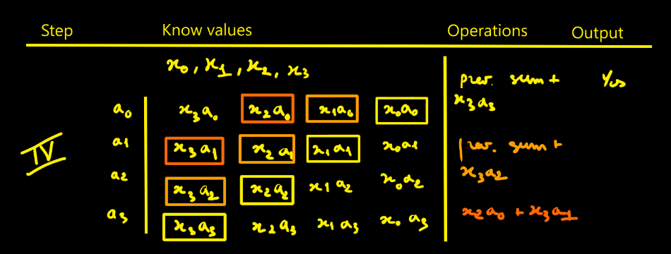
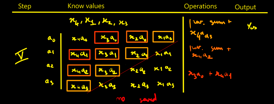
I thought designing the FIR filter would be simpler -  in fact it isn’t that straightforward. To picture how data flows through the filter, I drew tables showing successive cycles with the propagation of values and the operations done at each step. The filter parameters are noted a_i. The data to process are x_i. Here we choose N = 4 for illustration.

I started with a direct approach, the way you’d do it on an MCU. You’ll see it’s probably not the right method here.

Per modulus m_i, the FIR is:
y_i[n] = ( Σ_k=0…N−1 h_i[k] · x_i[n−k] ) mod m_i, for all i in [1, p]

Reconstruction by CRT:
y[n] = CRT( y₁[n], y₂[n], …, y_p[n] )

To escape purely sequential thinking, it helps to reason in terms of a production line: separate “lines” manipulate data items, cycle after cycle, as in a factory.

Moreover I count the operations and accumulations involved in an FIR with N taps and it easier to do with the following tables:

• N−1 additions
• N multiplications
• N cycles of latency (here one “cycle” means the time to ingest one full sample into the FPGA. The input sample is 16-bit, the input bus is 8-bit, so it takes 2 clocks to advance one cycle.)
• Looking at the step-5 table, we need to realize N + (N−1) + (N−2) + … + 1 = N(N+1)/2 intermediate products to fill the pipeline.
• We need to keep N products
• We also need to keep N−1 partial sums (accumulators)

Step-by-step

This is the direct approach. Of course, you must replicate that whole pipeline for each modulus. With k moduli, you duplicate it k times — that’s exactly where RNS parallelism comes from.

From the direct form to parallel and transposed architectures

While analyzing the cycle-by-cycle behavior of the direct form through these tables, a structural issue appears: for an FIR of N taps, the pipeline must effectively include N differentiated phases. At each cycle, every coefficient must be paired with its corresponding delayed sample — which requires a time-varying addressing scheme within the delay line.

As a result, the pipeline is not stationary: its internal data paths evolve from one cycle to the next (with a global sequence of N cycles). This makes programmation and sequencing heavier.

In addition to this non-stationary addressing, the addition chain itself must be broken into multiple intermediate stages to meet timing constraints. Together, these factors make the pipeline hard to program and tune.

Hence the natural question: isn’t there a more regular structure, where each pipeline stage would perform exactly the same operation at every instant?

Parallel direct form (fully parallel direct FIR)

If one wants a “hard” (stationary) pipeline, the solution is to let the samples slide through a delay line:
X₃ ← X₂ ← X₁ ← X₀ ← x[n].

The multipliers always see the correct positions (x[n], x[n−1], x[n−2], …): no more dynamic addressing.

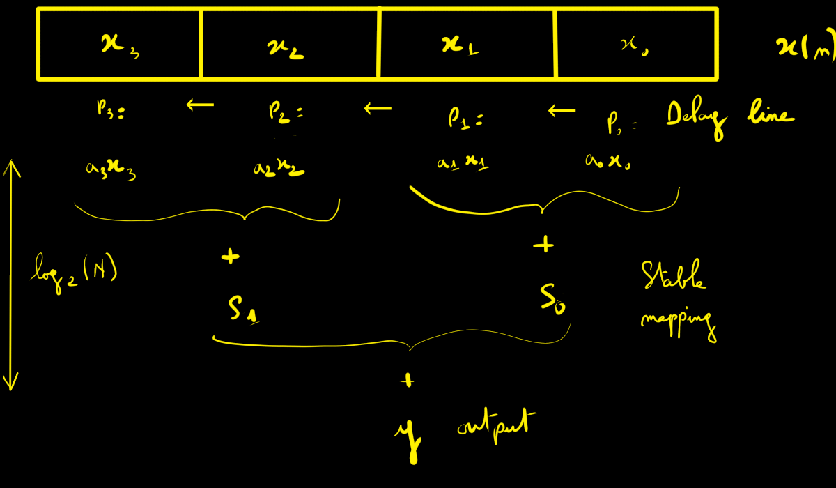
That’s much better — but there’s still a hard point:

• the reduction of N products (modular addition tree) must itself be pipelined;
• otherwise, the final addition becomes heavy and limits f_max.

Pipelining this reduction introduces a few extra cycles of latency. In practice, if one addition combines two values, the reduction tree has log₂(N) stages. With a ternary adder (three inputs), this drops to roughly log₃(N).

This approach is scalable for frequency if the addition tree is balanced and pipelined (depth ≈ log₂ N). Ressources needed linear growth (N multipliers, ~N additions, and delay-line registers).

This approach is often preferred for large filters: short pipeline latency (≈ log₂ N), easy routing (tree fan-in), and a fully stationary structure.

Transposed pipeline (transposed / systolic form)

Another possible structure is the transposed form. It consists of a chain of identical cells, each performing a multiply–add (mod) operation followed by a register. In this configuration, every stage executes the same operation at each clock cycle, making the pipeline extremely regular. Once the pipeline is primed, it delivers one output per cycle (the same for parallel direct form) and typically achieves a very high operating frequency for small to medium filter sizes.

We reuse the same setup with N = 4 coefficients {a₀, a₁, a₂, a₃}.
In the transposed form, the input sample x[n] is broadcast to all four multipliers. Each cell performs a multiply–add (mod m_i) followed by a register that stores the running sum for the next cycle.

The internal registers are R1, R2, and R3. All operations below are taken mod m_i.

y[n]  = a₀·x[n] + R1
R1'   = a₁·x[n] + R2
R2'   = a₂·x[n] + R3
R3'   = a₃·x[n]

After four cycles the pipeline is primed; from then on, one valid output is produced at every clock cycle. Each stage repeats the same operation at every cycle, which keeps timing and routing highly regular. 

However, as N increases, a technological limitation appears: the input sample x[n] must be broadcast to all N multipliers in parallel. This high fan-out can degrade both f_max and routing quality unless the distribution network is segmented or pipelined.

In contrast, the parallel direct form only feeds x[n] into the first register of the delay line, and the data then propagates by simple shifting—an architecture that scales much more gracefully for large N.

RNS context — and my choice

Since my goal is to exploit the Residue Number System (RNS) to push dynamic range and build deep FIR filters (large N), the RNS approach shows its full advantage when the filter depth is high.

For the next steps of this project, I will therefore focus on the fully parallel direct form: it offers a short pipeline latency, routing better suited to large N (no massive fan-out at input), and a stationary pipeline structure.

In the next log, I’ll present the implementation for the parallel direct approach with N = 64.