Applying these ideas: a PID controller  

At the beginning of our project, we talk about calculus as being useful to understand how things move and change.  Often we want to control how things move and change in a predictable way. One extremely common way of doing that is with a PID controller, which stands for “proportional-integral-derivative.”

Historically these were analog devices, and now are algorithms, that attempt to control something to a set value by using a mix of the current value, its integral (the sum of its value for some period in the past, effectively a smoothed past value) and its derivative (how fast, and in what direction, it is changing).

PID controllers are often correcting for some type of systematic error – friction, cooling, etc. They take data on some regular interval (“sampling”) and use how much that signal differs from a desired set value (the “error”) to send an adjustment to whatever it is they are measuring. For example, if something was trying to hold a temperature at 200 degrees and it measured 199 one sample ago and 201 now, the error one time step in the past would be -1 and now would be 1.

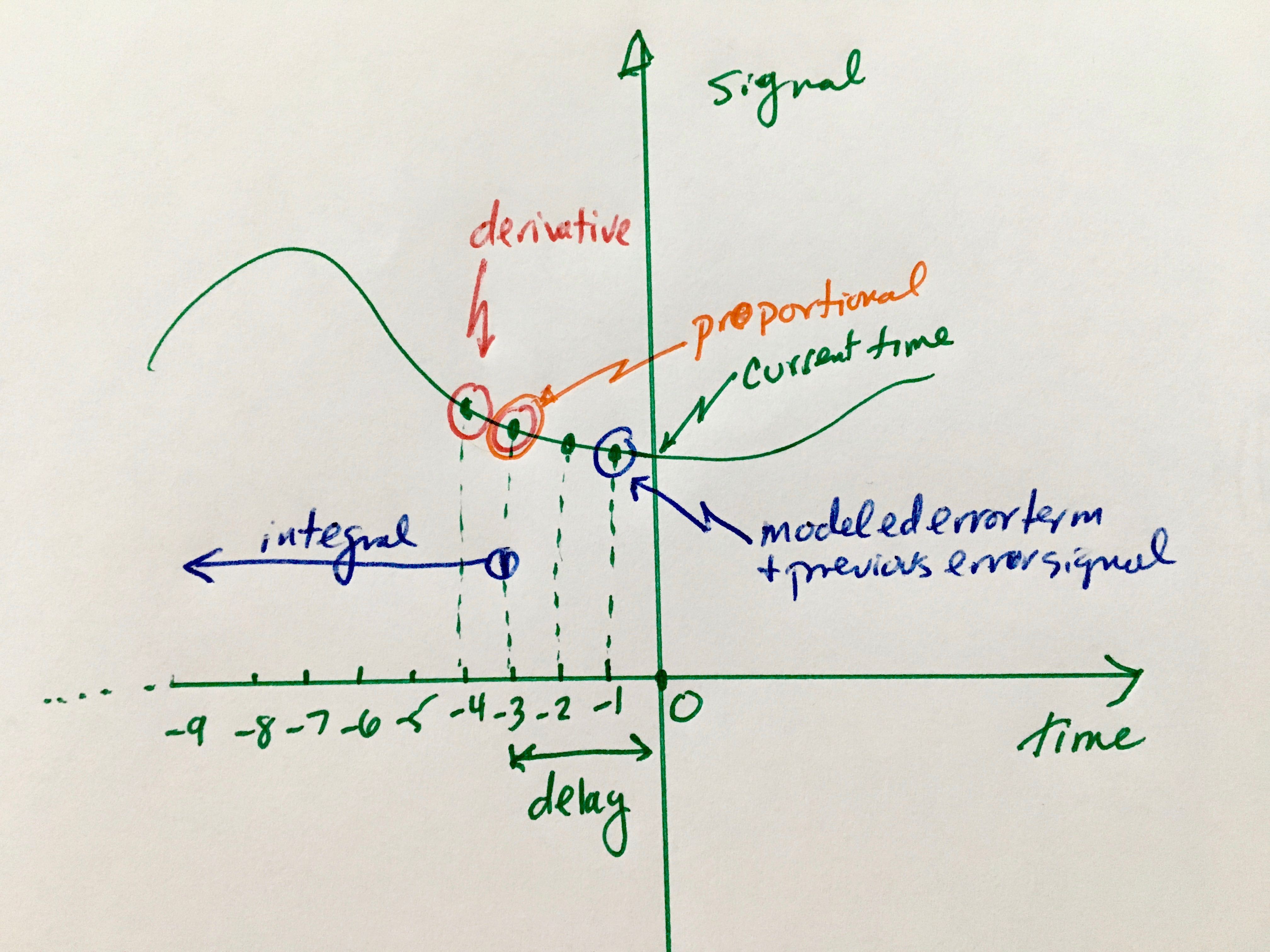
However, it’s a little trickier than that. There is a finite delay as the signal propagates through the system from the controller’s output back to its input. Let’s say that this delay is 3 time samples, for the sake of illustration. Then the inputs to calculate the next error signal that the controller will use are taken at the array of times shown in the picture.

Graph showing which time steps are used for each algorithm

The derivative term allows the controller to react to short-term errors that take the system too far away from its set point. The integral balances that out by essentially tracking any long-term systematic bias in the system, and correcting for it. If the terms are out of whack, a system might oscillate around or go unstable.

To write is as a sort-of equation:

Error (now, time=0) =         
      Error at the previous time sample (time = -1)

   + Kp * the error back one delay time ago  (time = -delay)

   + Ki * Integral of the error, based on a time range from the current time minus the delay back to as far back as the design accumulates (time = - delay back to whenever the controller turned on

    + Kd * Derivative, based on the signal value at times –delay and (–delay-1)

   + a modeled systematic outside error (a steady drift, sinusoidal noise, etc.)

Kp, Ki, and Kd are constants that can be created semi-empirically or based on a model of the system being controlled evaluated at time step -1.

PID controllers are everywhere, and have been around in some form or another for hundreds of years (for a history, see https://en.wikipedia.org/wiki/PID_controller.) Christian Huygens created a mechanical predecessor around the same time that Newton was working on calculus -- a “centrifugal governor” to manage how much grain was milled by a windmill as the windspeed changed. Nicholas Minorsky is credited with being the first person to write down the relevant math in 1922.

Numerical derivatives and integrals

We thought it would be interesting to find a way to model and view a simulated PID controller. In our integral and derivative models so far, we’ve just used the equations for a curve and its integral and derivative, which we figured out the traditional algebraic way. However, here, we do not have an actual function, so we need to integrate and differentiate in a discrete way. We could have done our curve-and-its-differential/integral models that way too, and we will probably create a generalized version there too.

At any rate, there are a lot of ways to do discrete derivatives (more usually called “finite differences”) and integrals. For now, we are using the most simple-minded way. That is, for a derivative of a curve we use the difference of the values of the curve at the most recent two time points. We should be dividing by the time step between when these were taken, but we since we are scaling everything by arbitrary scaling factors anyway we will assume the time between samples

For the integral, we recursively add on the value of the most recent time step to the sum thus far of all time steps.

There are other formulas that use more time steps or other corrections, but we will worry about those things later. A lot of calculus is festooned with special cases and ways to deal with the fact that not everything works all the time. We think that delving into that too soon is what makes “normal” calculus classes impenetrable. (As an aside for calculus teachers reading this, consider having your students consider the errors and failure modes of these (over) simplified lookback strategies.)

PID model

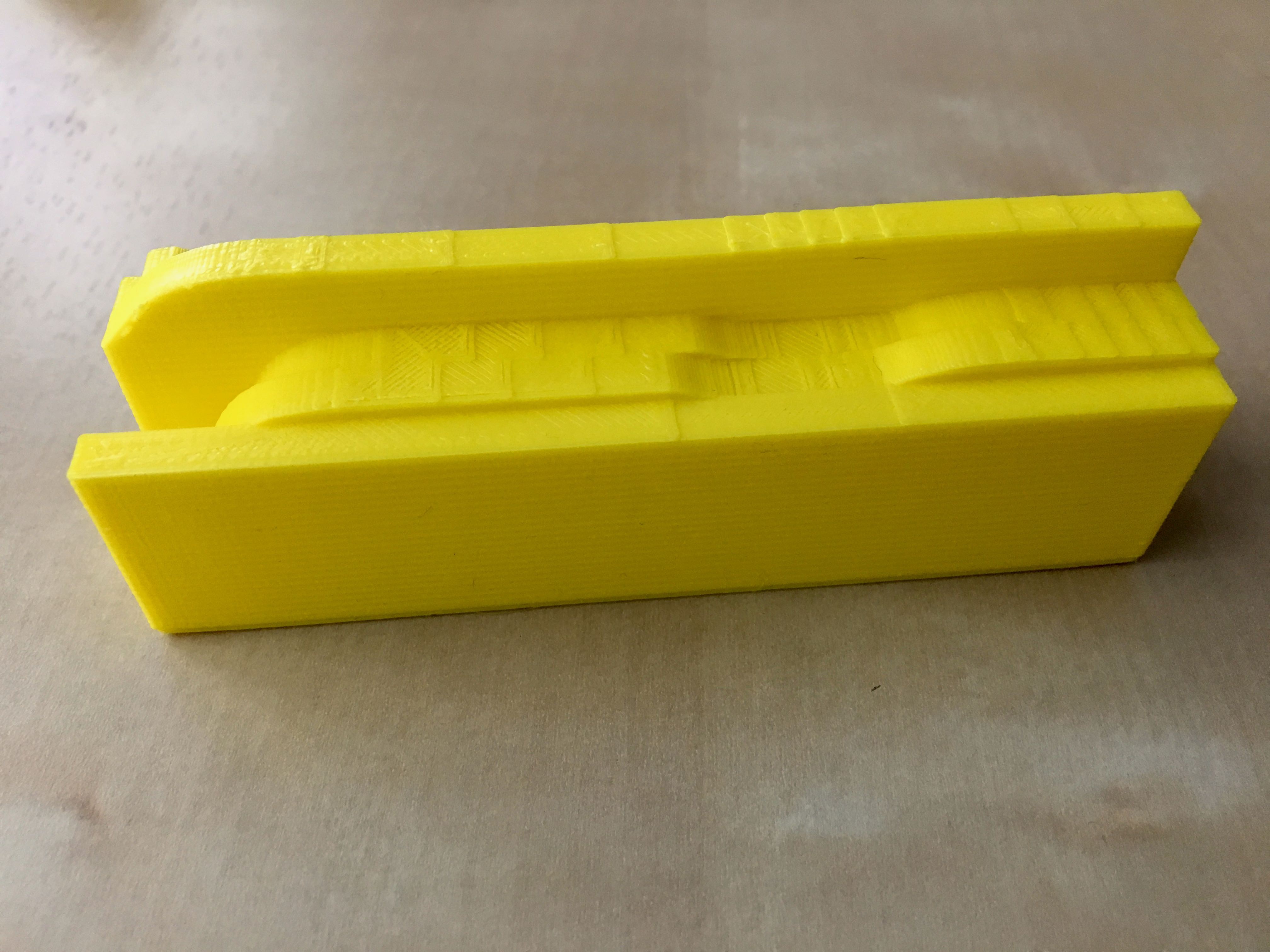
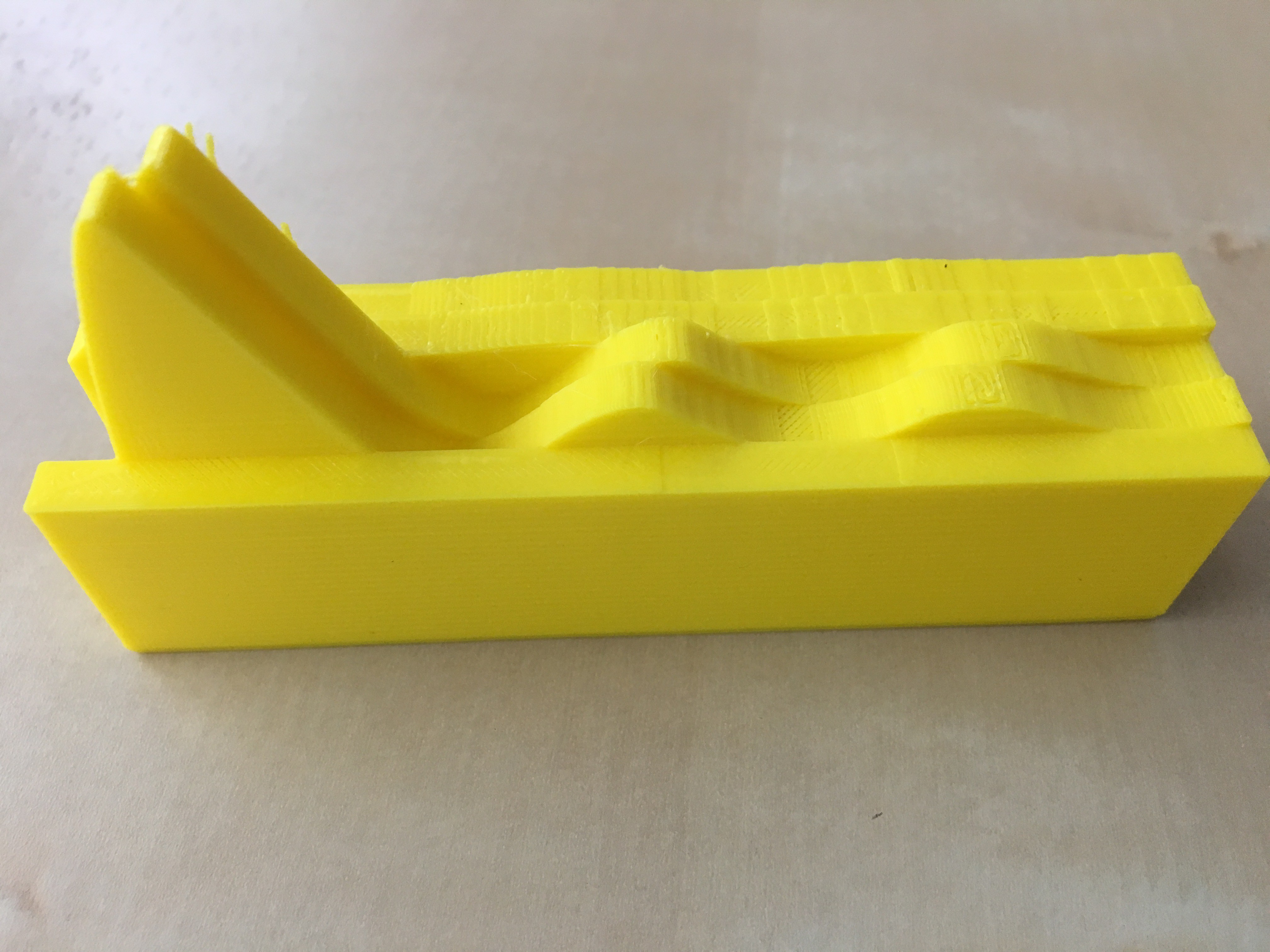
We have created two different PID controller models, and are printing side-by-side the time values of an input noise signal, the error (correction) signal, and the three P-I-D terms (the proportional term, the integral term, and the derivative term).

We designed one to go quickly to the desired steady state, and another to be somewhat unstable.

In the photos, time goes from left to right. Closest to you is the simulated system bias (a constant drift plus a small sinusoidal offset). Next is the error signal we are calculating from summing all these inputs; then the same function time shifted one delay time; then the integral and the derivative. They are all multiplied by scaling factors to be visible; in reality, some of these inputs would be very small.

PID controller terms graph for stable systemPID controller terms graph, unstable system

Obviously, you could also graph these curves and look at them all as colored lines on a 2d graph. But we find the third dimension adds some insight and interest.

This is one very specific example of an equation involving a mix of integrals, derivatives and other terms. There are many of these that govern important phenomena.  We want to see if there are ways to make combining terms more intuitive, or predicting types of solutions. Currently math students learn a large “toolbox” of these equations and what to do with them, but maybe we can take a more physical approach.

The 3D printable STL files will be included in the FILES section of this project. These were generated in OpenSCAD.  These are very much a work in progress and we are thinking about better methods for various aspects of this. But at least you can create and think about these particular ones  if you’d like.

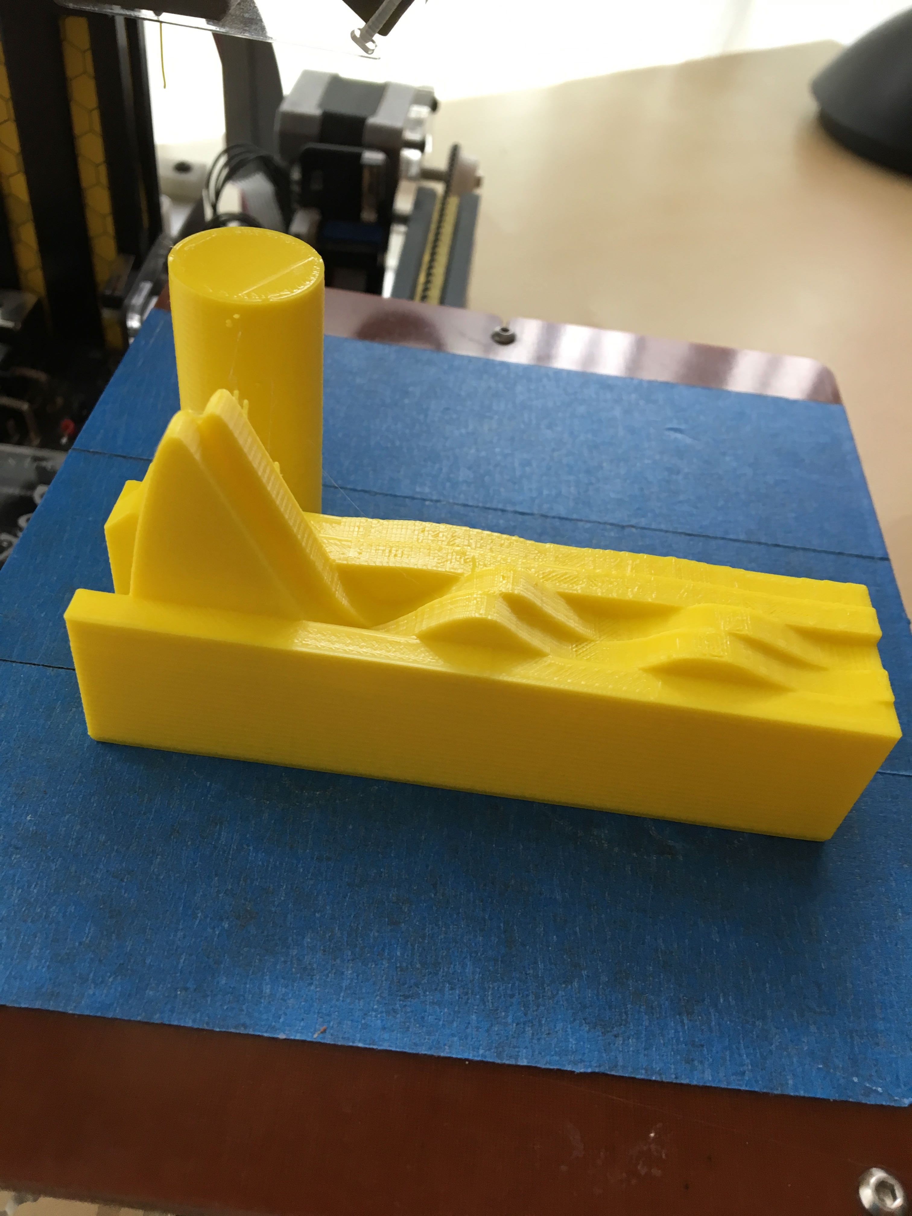
A final note: printing the second file was a challenge. It was printed as shown, and we used a cooling tower in the end to get the points to print correctly. See the photo below of the layout on a Bukito.  A cooling tower is just a cylinder that is a little taller than a delicate point on a print. It keeps the printer from trying to lay up plastic faster than it can cool and minimizes gloppy points on a print.  Note that we scaled the print down by 50% from the size is is in the STL.

PID print with a cooling tower