Project Details

We can use the FPGA to do fast numerical integration to solve differential equation models of neurons. This page describes a couple of neuron models and their solution by DDA techniques. Eugene Izhikevich developed a simple, semiempirical, model of cortical neurons. There are two state variables for each neuron: v is the membrane potential and u is the membrane recovery variable. The differential equations, parameter settings and examples of model output are shown in

http://people.ece.cornell.edu/land/courses/ece5760...

with a figure from Izhikevich's web site.

Implementation on the CycloneII FPGA
The model consists of several verilog modules which include (see also Ruben Guerrero-Rivera, et al below):

• Soma model (cell body and spike generator)
  • Time constant of 16 time steps (nominal time step of 1/16 mSec)
  • Square-law dynamics (as explained in the History section below)
  • Settable a, b, c, d, and I parameters (as explained in the diagrams above)
• Spike propagation delay (axon)
  • Delays of 1 to 64 time steps to simulate movement of a spike along an axon connection.
• Chemical Synapse
  • Constant current source gated by an presynaptic action potential.
  • Exponential fall time constant settable at 4, 8, 16, 32, 64, 128, 256 time steps.
  • Synaptic weight settable between -1 (inhibitory) and +1 (excitatory).
  • Input to daisy-chain current from another synapse module or from a constant current bias.
• Electrical Synapse
  • Current determined by a conductance and the voltage difference between two cells.
  • Rectifying (foward or backward) and symmetrical versions available.
  • Input to daisy-chain current from another synapse module or from a constant current bias.
• Spike time dependent plasticity (STDP) learning unit to be attached to a synapse.
  • The module changes the weight of a synaptic connection depending on whether the postsynaptic spike follows (causal) or leads (non causal) the presynaptic input spike. Causal connnections are made stronger, noncausal weaker.
  • Exponential spike intereaction time constant settable at 4, 8, 16, 32, 64, 128, 256 time steps
  • The delta-weights for causal and noncausal changes are settable, as are an initial weight and a maximum weight.

Two reciprocal pairs with electrical synapse between them.
The top-level module (and project archive) instantiates 4 neurons with the following connections:

1. Neuron 1 spike output is connected to
   1. Neuron 2 through a synapse with weight -0.016
   2. Neuron 3 through an electrical synapse with rectification and a conductance of 1/64. Current flow occurs only if v1>v2.
   3. LED 1
2. Neuron 2 spike output is connected to
   1. Neuron 1 through a synapse with weight -0.016
   2. LED 2
3. Neuron 3 spike output is connected to
   1. Neuron 4 through a synapse with weight -0.016
   2. Neuron 1 through an electrical synapse with rectification and a conductance of 1/64. Current flow occurs only if v1>v2.
   3. LED 3
4. Neuron 4 spike output is connected to
   1. Neuron 3 through a synapse with weight -0.016
   2. LED 4

The two pairs of cells sync up because the weak excitatory coupling provided by the electrical synapse tend to make cells 1 and 3 fire at the same time. Note that the electrical synapse module needs to know the voltage in both cells and can inject current into both cells.

Reciprocal pair with STDP-modifed synapse to a third neuron
The top-level module (and project archive) instantiates 3 neurons with the following connections:

1. Neuron 1 spike output is connected to
   1. Neuron 2 through a synapse with weight -0.016
   2. Neuron 3 through a synapse with STDP and an initial weight of zero. The STDP weight increments are adjusted so that the firing of neuron 3 eventually syncs up with neuron one.
   3. LED 1
2. Neuron 2 spike output is connected to
   1. Neuron 1 through a synapse with weight -0.016
   2. LED 2
3. Neuron 3 spike is not used, just sent to LED 3 for monitoring

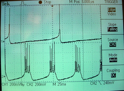
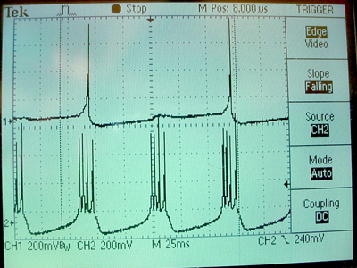
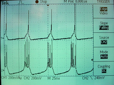
The three images below show the initial, unsynced voltages (neuron 1 on bottom, neuron 3 on top), an intermediate state, and the final conveged state generated by the verilog module above. Initially, both neurons are spontaneously active, but with zero synaptic connection weight between them. The Hebbian synapse is adjusted so that after a few thousand spikes, the coupling between cells slowly developes. In the intermediate state you can see that every other burst of neuron 1 is triggering a spike in neuron 3, but you can also see the small voltage generated by a subthreshold coupling. The final, equlibrium state shows one spike in neuron 3 for every burst in neuron 1.

References

• Ruben Guerrero-Rivera, et al, Programmable Logic Construction Kits for Hyper-Real-Time Neuronal Modeling, Neural Computation, Volume 18 , Issue 11 (November 2006) Pages: 2651 - 2679
• Eugene M. Izhikevich , Simple Model of Spiking Neurons, IEEE Transactions on Neural Networks (2003) 14:1569- 1572