Bruce Land
Introduction
The following software was written to aid in the teaching of BioNB330, Introduction to Computational Neuroscience. The software is meant to clarify concepts introduced in lecture and to serve as the basis for homework assignments. The programs written are:
- Neural model. This program allows the student to:
- Select the current applied to a model neuron, including pulses, sinusiodal, and noise waveforms.
- Set the neuron to linear, sigmoid, or integrate-and-fire (spiking).
- Set the neuron threshold, time constant and input resistance.
- View the threshold, input current waveform, and membrane voltage waveform.
- Measure times and amplitudes from the simulated time course.
- Produce an interspike interval histogram, if the neuron is in spikeing mode.
- Receptive field tuning. This program allows the student to:
- Set three "visual" input neurons, each with its own sinusiodally varying response to the angle of a rotating line. The optimal angle, amplitude of response, and zero offset may be chosen.
- Set the weight of connnection of each of the three neurons to an output neuron.
- Lateral Inhibition. This program is an extension of the previous program and allows:
- Set three "visual" input neurons, each with its own sinusiodally varying response to the angle of a rotating line. The optimal angle, amplitude of response, and zero offset may be chosen.
- Set the weight of connnection of each of the three neurons to each of three linear neurons.
- The second-level, linear neurons have optional cross-coupling and variable weights to a linear output neuron.
- Two cells with inputs and cross-coupling. This program alllows the student to:
- Select the current applied to two model neurons, including pulses, sinusiodal, and noise waveforms and output for the other cell.
- Set the neurons to linear, sigmoid, or integrate-and-fire (spiking).
- Set the neurons time constant and input resistance.
- Linear Association Learning. This program allows the student to:
- In learning mode: choose a binary input and output pattern, then increment the weights of the association matrix.
- In recall mode: choose a binary input. The association matrix is used to compute an output.
- Change the threshold used to set the outputs.
- Hebbian Learning. This program allows the student to:
- In learning mode: The program associates the inputs of five cells (with overlapping receptive fields) with an unconditioned stimulus. The effect is to increment the weights of of the connections between the input cells and the output cell..
- In sweep mode: The program sweeps throuugh all possible stimuli and produces a curve of the output amplitude based on the connection weights and an optional output threshold..
- The student can vary various learning parameters.
- Auto-Associative Learning
- A 2D binary pattern can be clicked into 25 input units. Each input unit is also an output unit.
- The connection scheme between units is all-to-all, so there are 625 weights for 25 units.
- After patterns have been stored, the recall function will attempt to complete an imcomplete input pattern.
Using the Neural model program
This program helps the student investigate simplified, computational models of neurons. The program requires Matlab 6.1 or later to run. Download the program by right-clicking on the above program link.
The user interface is shown below. In summary, you can:
- set up inputs to a model neuron
- choose the membrane parameters (resistance, time constant, threshold)
- choose the simulated output mechanism (spiking, sigmoid)
- run the simulation
- stop the simulation to measure outputs
- construct an interspike interval histogram (if in spike mode).
Each interactive control will be explained in following paragraphs. The mathematical basis for the model is explained on a separate page.
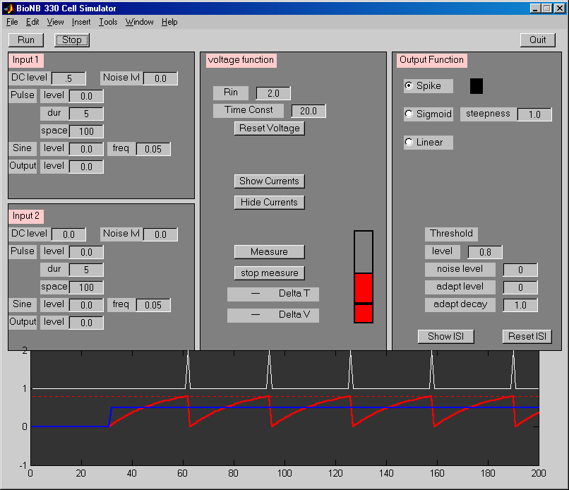
Input Sections
There are two inputs to the simulated neuron, each with its own controls. Each input acts as a current-input with a waveform determined by the control settings:
- The
DC leveledit field sets a steady, unchanging current. The default setting when the program starts is for all inputs to be zero. You can set the DC input to amplitude 0.5 to cause spikeing when you pressRun. This level is sufficient to cause output spikes initially. The useful range is -1 to +1. Negative currents are inhibitory, positive are excitatory. - The
Noise Lvledit field sets the amplitude of a random current. This can be used to simulate synaptic noise. The useful range is 0 to +1. - The
Pulseinput allows current pulses to be applied the the model neuron, simulating currents caused by action potentials. Pulses have three associated edit fields:levelsets the amplitude of the pulse. Useful range is -1 to +1.durationsets the time the pulse lasts. Useful range is 1 (time step) to 100 or so.spacesets the time between pulses. Useful range is 1 (time step) to 1000 or so.
- The
Sineinput allows sinusoidally varying currents to be applied the the model neuron, simulating currents caused by smoothly varying sensory inputs. The sine function has two associated edit fields:levelsets the amplutide of the wave. Useful range is -1 to +1.frequencysets the rate at which the current changes. Useful range is .001 (1 cycle per 1000 time steps) to 0.5 (one cycle per 2 time steps).
- The
Outputinput allows the output of the simulated neuron to feed back to the input. The level control sets the amount of feedback.The useful range is -1 to +1.
Voltage Function Section
The Voltage Function section sets the membrane parameters, and also allows for measurements and monitoring the details of membrane current. The red bar animates the current membrane voltage, while the box surrounding it animates the threshold (if the threshold changes). There are two subthresold membrane parameters:
- The
Rinedit field sets the input resistance of the neuron. A higherRinimplies that the applied current will cause a bigger voltage change (since E=IR). The useful range is 0.5 to 10 or so. - The time constant field sets the time over which the neuron will summate current. A value of 1 implies that the voltage exactly follows the instantaneous value of the current. A time constant of 1000 or so means that the current will summate for a 1000 time steps.
- Pressing the
Voltage Resetbutton will force the voltage to resting potential.
Clicking the Measure button stops the simulation. When you click the mouse button in the waveform display, a diamond marker is placed on the screen. This becomes the zero-point for the measurement. As you move the mouse, the difference between the position of the diamond and the position of the mouse is used to calculate a voltage and a time.
Output Function Section
The Output Function section sets the type of neuron (spiking/sigmoid) and the threshold for output. There are also controls for displaying and reseting the interspike interval (ISI) histogram. The neuron can be in one of two output modes:
- In spike mode, the membrane voltage resets to zero when the voltage is greater than the threshold, and a spike is generated.
- In sigmoid mode, the output is a nonlinear, continuous function of the voltage. The function is Vn/(Vn+Tn), where V is the membrane voltage and T is the threshold. This function is always zero if V=0 and is one if V>>T. You can set the steepness of the function by increasing n. The shape of the sigmoid is displayed in a small animated window.
- In linear mode, the ouitput is given by:
- zero if V<threshold
- V-threshold if V>threshold
The threshold may be modified in various ways:
- The level can be set. The useful range is 0.1 to 1.
- Noise can be added to the threshold to simulate random, small fluctuations in the neuron. The useful range is 0 to 0.5.
- The threshold can be made to vary after a spike to simulate relative refractory period.
If the neuron is in spike mode, the ISI controls may be used to display an interspike interval histogram. The Reset ISI button clears the spike memory.
Using the Receptive Field model program
This program helps the student investigate a simple receptive field model. The program requires Matlab 6.1 or later to run. Download the program by right-clicking on the above program link. Three sensory inputs drive one output neuron. The three inputs have user-selectable responses to a rotating line. When the line rotates through the receptive field of an input, that input generates a current. The currents are summed at the output neuron to form a response to the rotating line. The line rotates from 0 to 180 degrees, then stops.
The user interface is shown below. In summary, you can:
- set up inputs to a model neuron
- choose the membrane parameters (resistance, time constant, threshold)
- choose the simulated output mechanism (spiking, sigmoid, linear)
- run the simulation
- stop the simulation to measure outputs
- construct an interspike interval histogram (if in spike mode).
- show each input current in a different color, and total current in white.
Each interactive control will be explained in following paragraphs.
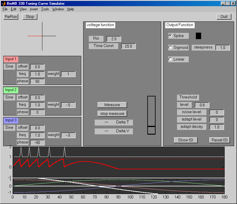
Input Sections
There are three inputs to the simulated neuron, each with its own controls. Each input acts as a current-input with an line-angle dependent waveform determined by the control settings:
- The
Offsetedit field sets the average current of the sinewave input. The default setting when the program starts is for al offsets to be 0.0. The useful range is -1 to +1. A setting of zero means that the the sinewave will be excitatory for the positive half-cycle and inhibitory for the negative half-cycle. A setting of +1 means that the entire sinewave will be excitatory. A setting of -1 means that the entire sinewave will be inhibitory. Negative currents are inhibitory, positive are excitatory. - The
Frequencyedit field sets the number of maxima in the input response curve. A frequency of 1 corresponds to one maximally stimulating angle of the line (per revolution) as it rotates. The useful range is 1 to 4. - The
Phaseinput sets the value of the best angle for stimulating an input. - The
weightinput sets the strength of the current applied to the neuron.
The initial control settings are shown in the figure above.
Voltage Function Section
The Voltage Function section sets the membrane parameters, and also allows for measurements and monitoring the details of membrane current. The red bar animates the current membrane voltage, while the box surrounding it animates the threshold (if the threshold changes). There are two subthresold membrane parameters:
- The
Rinedit field sets the input resistance of the neuron. A higherRinimplies that the applied current will cause a bigger voltage change (since E=IR). The useful range is 0.5 to 10 or so. - The time constant field sets the time over which the neuron will summate current. A value of 1 implies that the voltage exactly follows the instantaneous value of the current. A time constant of 1000 or so means that the current will summate for a 1000 time steps.
Clicking the Measure button stops the simulation. When you click the mouse button in the waveform display, a diamond marker is placed on the screen. This becomes the zero-point for the measurement. As you move the mouse, the difference between the position of the diamond and the position of the mouse is used to calculate a voltage and a time.
Output Function Section
The Output Function section sets the type of neuron (spiking/sigmoid) and the threshold for output. There are also controls for displaying and reseting the interspike interval (ISI) histogram. The neuron can be in one of two output modes:
- In spike mode, the membrane voltage resets to zero when the voltage is greater than the threshold, and a spike is generated.
- In sigmoid mode, the output is a nonlinear, continuous function of the voltage. The function is Vn/(Vn+Tn), where V is the membrane voltage and T is the threshold. This function is always zero if V=0 and is one if V>>T. You can set the steepness of the function by increasing n. The shape of the sigmoid is displayed in a small animated window.
- In linear mode, the ouitput is given by:
- zero if V<threshold
- V-threshold if V>threshold
The threshold may be modified in various ways:
- The level can be set. The useful range is 0.1 to 1.
- Noise can be added to the threshold to simulate random, small fluctuations in the neuron. The useful range is 0 to 0.5.
- The threshold can be made to vary after a spike to simulate relative refractory period.
If the neuron is in spike mode, the ISI controls may be used to display an interspike interval histogram. The Reset ISI button clears the spike memory.
Using the Lateral Inhibition model program
This program helps the student investigate a receptive field model with coupling between cells. The program requires Matlab 6.1 or later to run. Download the program by right-clicking on the above program link. Three sensory inputs each drive one second-layer neuron. The three second-layer neurons may be cross-coupled and/or drive an output neuron. The three inputs are similar to the previous program. The second-layer neurons and output neuron have linear response to input current (above a settable threshold).
The user interface is shown below. In summary, you can:
- set up inputs to three model neurons
- choose the membrane parameters (threshold)
- run the simulation. The simulation runs from 0 to 180 degrees, then stops.
- stop the simulation to measure outputs
- Select which of the voltage plots you wish to view. Plots are color-coded to match the colors on the tabs associated with inputs and cells.
Each interactive control will be explained in following paragraphs.
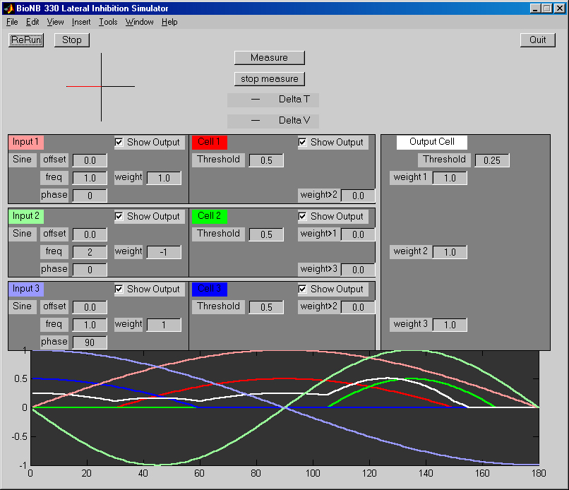
Input Sections
There are three inputs to the simulated neuron, each with its own controls. Each input acts as a current-input with an line-angle dependent waveform determined by the control settings:
- The
Offsetedit field sets the average current of the sinewave input. The default setting when the program starts is for al offsets to be 0.0. The useful range is -1 to +1. A setting of zero means that the the sinewave will be excitatory for the positive half-cycle and inhibitory for the negative half-cycle. A setting of +1 means that the entire sinewave will be excitatory. A setting of -1 means that the entire sinewave will be inhibitory. Negative currents are inhibitory, positive are excitatory. - The
Frequencyedit field sets the number of maxima in the input response curve. A frequency of 1 corresponds to one maximally stimulating angle of the line (per revolution) as it rotates. The useful range is 1 to 4. - The
Phaseinput sets the value of the best angle for stimulating an input. - The
weightinput sets the strength of the current applied to the second-layer neuron. - The
show outputcheckbox shows/surpresses this current.
Cell Sections
The Cell sections sets the membrane threshold and the cross-coupling weights from each second-layer cell to its neighbors.
- The threshold sets the level at which the cell starts to respond linearly. The useful range is 0 to 1.
- Cross-coupling weights between layer-two cells. the useful range is about -1 to +1.
- The
show outputcheckbox shows/surpresses this voltage.
Clicking the Measure button stops the simulation. When you click the mouse button in the waveform display, a diamond marker is placed on the screen. This becomes the zero-point for the measurement. As you move the mouse, the difference between the position of the diamond and the position of the mouse is used to calculate a voltage and a time.
Output Cell Section
The Output Cell section sets the threshold for output and the input weights from each of the layer-two neurons. The useful ranges are as above.
Using the Two Cell model program
This program helps the student investigate two interconnected model neurons. The program requires Matlab 6.1 or later to run. Download the program by right-clicking on the above program link. There are a variety of input options to each cell, including connection to the output of the other cell.
The user interface is shown below. In summary, you can:
- set up inputs to two model neurons
- choose the membrane parameters (resistance, time constant, threshold)
- choose the simulated output mechanism (spiking, sigmoid, linear)
- run the simulation
- stop the simulation to measure outputs
- construct an interspike interval histogram (if in spike mode).
Each interactive control will be explained in following paragraphs.
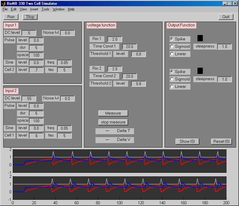
Input Sections
There are two input sections corresponding to the two simulated neuron, each with its own controls. Each input acts as a current-input with a waveform determined by the control settings:
- The
DC leveledit field sets a steady, unchanging current. The default setting when the program starts is for Input 1 to have a steady current of amplitude 0.5. This level is sufficient to cause output spikes initially. The useful range is -1 to +1. Negative currents are inhibitory, positive are excitatory. - The
Noise Lvledit field sets the amplitude of a random current. This can be used to simulate synaptic noise. The useful range is 0 to +1. - The
Pulseinput allows current pulses to be applied the the model neuron, simulating currents caused by action potentials. Pulses have three associated edit fields:levelsets the amplitude of the pulse. Useful range is -1 to +1.durationsets the time the pulse lasts. Useful range is 1 (time step) to 100 or so.spacesets the time between pulses. Useful range is 1 (time step) to 1000 or so.
- The
Sineinput allows sinusoidally varying currents to be applied the the model neuron, simulating currents caused by smoothly varying sensory inputs. The sine function has two associated edit fields:levelsets the amplutide of the wave. Useful range is -1 to +1.frequencysets the rate at which the current changes. Useful range is .001 (1 cycle per 1000 time steps) to 0.5 (one cycle per 2 time steps).
- The
Cell1 or Cell2input allows the output of the simulated neuron to feed back to the other cell. The level control sets the amount of feedback.The useful range is -1 to +1. Thetaucontrols set the time consant of the synaptic current.
Voltage Function Section
The Voltage Function section sets the membrane parameters, and also allows for measurements and monitoring the details of membrane current. The red bar animates the current membrane voltage, while the box surrounding it animates the threshold (if the threshold changes). There are two subthresold membrane parameters:
- The
Rinedit field sets the input resistance of the neurons. A higherRinimplies that the applied current will cause a bigger voltage change (since E=IR). The useful range is 0.5 to 10 or so. - The time constant field sets the time over which the neurons will summate current. A value of 1 implies that the voltage exactly follows the instantaneous value of the current. A time constant of 1000 or so means that the current will summate for a 1000 time steps.
- The threshold sets the point at which the cell voltage triggers an output.
Clicking the Measure button stops the simulation. When you click the mouse button in the waveform display, a diamond marker is placed on the screen. This becomes the zero-point for the measurement. As you move the mouse, the difference between the position of the diamond and the position of the mouse is used to calculate a voltage and a time.
Output Function Section
The Output Function section sets the type of neuron (spiking/sigmoid) and the threshold for output. There are also controls for displaying and reseting the interspike interval (ISI) histogram. The neuron can be in one of two output modes:
- In spike mode, the membrane voltage resets to zero when the voltage is greater than the threshold, and a spike is generated.
- In sigmoid mode, the output is a nonlinear, continuous function of the voltage. The function is Vn/(Vn+Tn), where V is the membrane voltage and T is the threshold. This function is always zero if V=0 and is one if V>>T. You can set the steepness of the function by increasing n. The shape of the sigmoid is displayed in a small animated window.
- In linear mode, the ouitput is given by:
- zero if V<threshold
- V-threshold if V>threshold
If the neuron is in spike mode, the ISI controls may be used to display an interspike interval histogram. The Reset ISI button clears the spike memory.
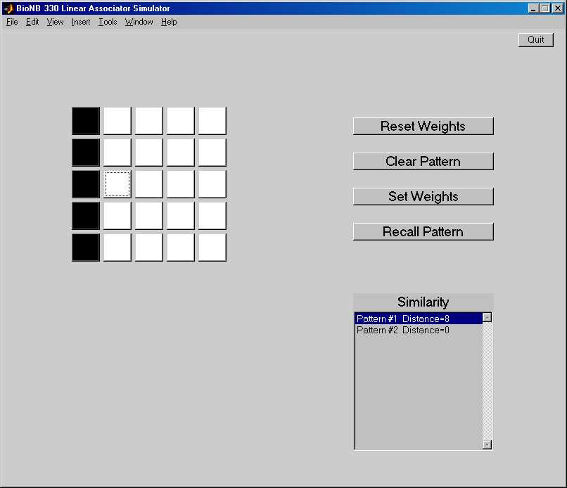
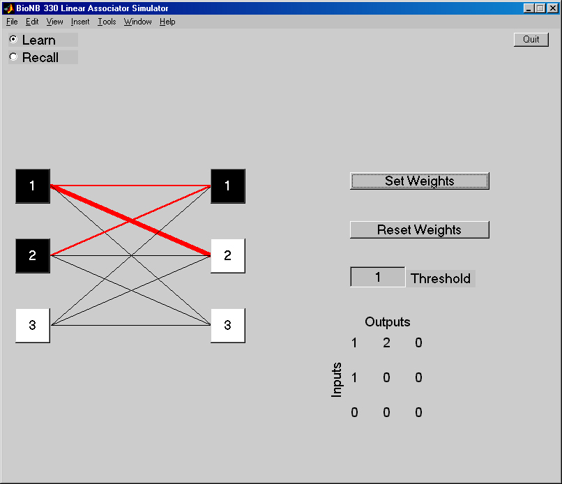
Linear Association Learning
This program helps the student investigate a simple learning algorithm. The program requires Matlab 6.1 or later to run. Download the program by right-clicking on the above program link. The user can associate output patterns with input patterns by clicking on the appropriate (binary valued) boxes.
- In
Learnmode, clicking on input units and output units toggles them from off (white) to on (black) and back. Once a pattern is set, theSet Weightsbutton will modify the association matrix shown at the lower right. The width of the lines connecting the inputs and outputs gives an estimate of the connection strength. - In
Learnmode, clicking on theReset Weightsbutton will zero all the weights. - In
Recallmode, clicking on input units toggles them from off (white) to on (black) and back. When an input pattern is set, an output is computed and displayed. TheThresholdedit field sets the level at which an ouput will be considered on (black).
Hebbian Learning
This program helps the student investigate a Hebbian learning algorithm. The program requires Matlab 6.1 or later to run. Download the program by right-clicking on the on the above program link.
- In
Learnmode, the program associates the inputs of five cells (with overlapping receptive fields, shown on the left of the image below) with an unconditioned stimulus. The effect is to increment the weights of of the connections between the input cells and the output cell, proportional to the product of activiy of the input and output cells. The width of the lines connecting the inputs and outputs gives an estimate of the connection strength. During training, the stimulus (red line at 1700 Hz) and unconditioned stimulus (green square) flash once for each reinforcement. - In
Learnmode, clicking on theResetbutton will zero all the weights. - In
Sweepmode, the program sweeps throuugh all possible stimuli and produces a curve of the output amplitude based on the learned connection weights and an optional output threshold. TheOutput Thresholdedit field sets the level at which an ouput will be considered nonzero. The color intensity of each input unit is proportional to its ouput value. - The student can set the learnng rate, the number of training trials and a Input threshold. The
Input Thresholdsetting allows the learning algorithm to ignore small inputs. There are four modes for normalizing the weights.
A slightly modified version of the program has a subtractive threshold for inputs, so that weights can become negative. There is a new control defined to set the initial weights to non-zero values.

Auto-association Learning
This program helps the student investigate a learning algorithm which allows pattern completion. The program requires Matlab 6.1 or later to run. Download the program by right-clicking on the above program link. The user can enter input patterns by clicking on the appropriate (binary valued) boxes.
- The
Set Weightsbutton computes weights for an input pattern, so that part of the input will tend to rrecall all of the pattern. - The
Recall Patternbutton, computes an output based on the current weights and inputs. - clicking on the
Reset Weightsbutton will zero all the weights. - clicking on the
Clear Patternbutton will zero all the input boxes. - The Similarity box indicated the distance of the current pattern from the stored patterns.