Let's have a look at a first pass at making a simulator for the coded field MRI.

Simulating an instrument is a helpful way to understand the design, how different elements interact, how the instrument behaves in the presence of noise, and identify any issues early on to help inform your design decisions. I have some experience with this from my first postdoc in designing an adaptive coded-aperture spectral imager, and so I've started putting together a simulator for the coded field MRI to help understand the design considerations, and what kind of performance one might expect with such a system with specific design decisions. The high-level and very powerful MATLAB numerical simulation suite is the standard tool for constructing these simulations, but in the spirit of open source I'll be using GNU Octave, an open-source effort at cloning much of MATLAB's functionality.

Some folks like to design all of the individual components of a system and then piece them all together at the end. I prefer to have a simple but modular system up and running end-to-end so that I can see how each new component affects the system, and get a better intuition of how things work. Here I've put together a very simple simulation that is idealized and doesn't yet incorporate many important physical phenomena, and so we'll progressively add them in over the course of the project as we get a better appreciation for them.

The basic questions that we might have at the beginning of this project are:

• How accurately do I have to measure the magnetic field of the code to arrive at accurate reconstructions?
• How many measurements will it take to reconstruct an image? How many different codes? (and, ultimately, how long will each slice (or volume) take to measure?)
• What is the relationship between the number of measurements and reconstruction quality?
• How does noise affect the reconstruction quality?
• How does the range of magnetic field intensities in the code field affect the number of measurements?
• How small will the magnetic resonance signal be? How sensitive would a receiver have to be to pick it up?
• What frequency range will the receiver have to be sensitive at, and what sampling rate will it have to have?

and many others. Here we'll begin to find answers to some of these.

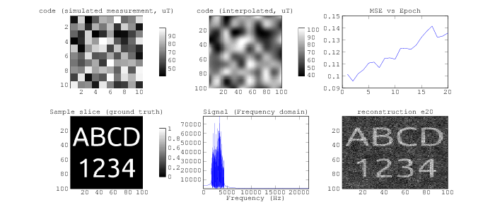
Let's orient to the simulator (above).

• Code (measured) (top left): Here we have a low-resolution simulation of the coded field, as measured from the magnetometer. This simulated code field is measured at a 10x10 resolution (to help ground this, you could think of it as 10cm x 10cm), and each "pixel" of this code is currently randomly generated to be between a certain range (say 40uT to 55uT). In practice, this will likely need to be much closer to a 1mm resolution, but it's helpful for visualizing. Random codes likely aren't physically realizable with whatever configuration of code field gradient coils we end up putting together, but random codes are popular in coded aperture imaging, so we'll start here.
• Code (interpolated) (top center): Here we make the assumption that the code intensity is slowly varying over distances that are smaller than the the measured code, and interpolate the measured code to a higher resolution to get a better map of the field intensities over our simulated sample.
• Sample (bottom left): Our simulated sample -- here just two dimensional, and a test pattern. In reality this would be the fruit, appendage, or other sample that you're trying to measure.
• Signal (bottom center): The simulated signal generated by the sample given the code field, after one magnetic resonance pulse (ie. placing the sample in a ~1T field, then quenching the field so that it quickly collapses down to the code field, and recording the signal produced). This signal is in the frequency domain.
• Reconstruction (bottom right): Our reconstruction of the sample, after a given number of measurements.

The simulator also includes a graph of the error in the reconstruction over time (top right), but I'm not sure that the metric I'm using now is well fit for this task, so we'll ignore it for now.

Before looking at some initial results, let's get an idea of the process, to help ground the ideas in the last post.

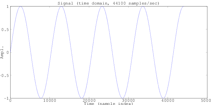
The magnetic resonance process from the proton precession magnetometer protocol causes the nuclei in a given spatial area to precess at a frequency determined by the magnetic field strength at their location. Assuming that the magnetic field strength is perfectly uniform, the signal might look something like this (above) -- a signal at one frequency. Note that physically has an exponential decay in it (the T2 relaxation), but here we're going to start with something exceedingly simple that doesn't decay, and add in a decay model later.

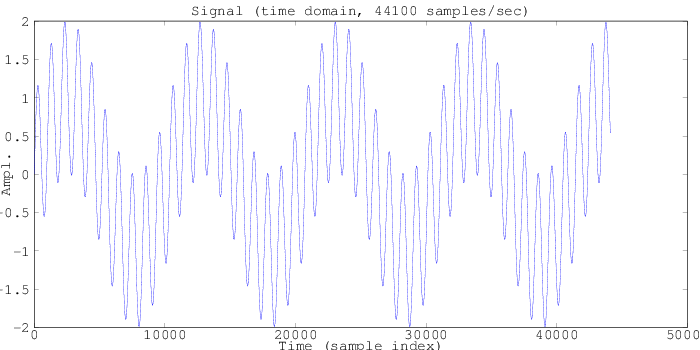
Now imagine instead of listening from only a single spatial location, we listen from two -- each having a different (but completely uniform) magnetic field strength. The signal might look something like this (above), with two frequencies -- one from each spatial location.

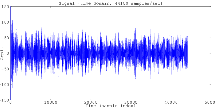
Extending this further to the 100x100 (10,000) points modeled in this simulation, we can see an absolute cacophony of 10,000 spatial locations all broadcasting their magnetic resonance signals at once. Here we'll switch to the frequency domain, where it's a little easier to make out the structure of this signal.

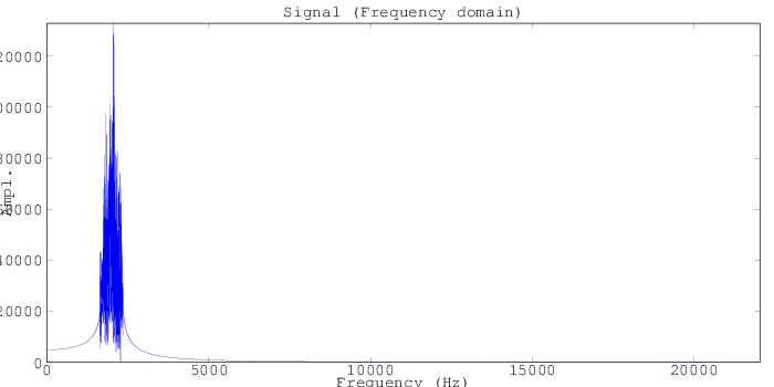
Here on the frequency domain plot we can see a large set of signals over a short band of frequencies around 2kHz, corresponding to random code intensities between 40uT and 55uT. Here, each frequency represents somewhere between one to a small number of spatial locations, and the amplitude represents the sum of the "signal" (say, the amount of water at a given location, represented by the intensity of the sample image).

Now, with a knowledge of what our code looks like, we can start to back out what the original sample looked like -- and that reconstruction will get better as we include more and more measurements with different codes.

Here's a first simulation, with the original sample (left), as well as the code (center) and reconstruction (right) as we progress from 1 to 20 measurements. At first the reconstruction is terrible, and looks very little like the sample -- but as we accumulate many measurements from different codes, the reconstruction starts to resemble the sample. This is because each code is full of ambiguities -- since the magnetic field intensity at a given spatial location could be the same as the intensity at another spatial location, the signal at a given frequency can't be accurately attributed to a given spatial location. One code might pool together spatial locations A and B into one frequency, so we can't tell how much came from A and how much came from B. But the next code might pool A and C into one frequency, and the next one A and D, and so on, and so after many measurements with many different (and known) combinations, we can start to back out what the signal from location A, and all the other locations, must look like.

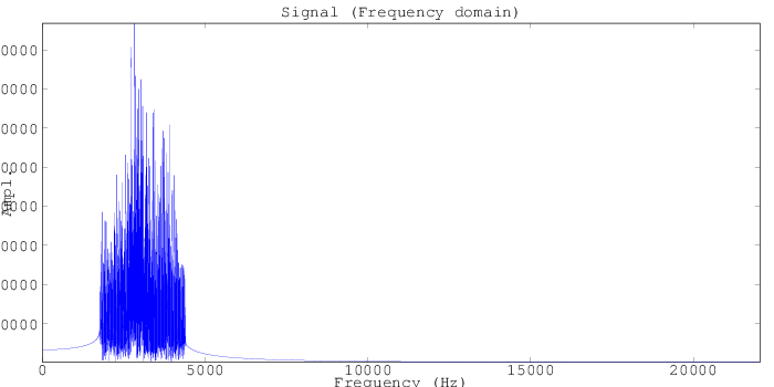
The last simulation was using only a very narrow range of magnetic field intensities in the code (40uT to 55uT), and so it had to pack a lot of information into a small band of frequencies. Let's increase the code range to between 40uT and 100uT (we're still in fridge magnet territory on these intensities), and see how this helps out our reconstruction. Above we can see that now our signal spans from between about 2kHz to 4kHz, which is still able to be well-sampled using our simulated sampling frequency of 44.1kHz (audio sampling rates).

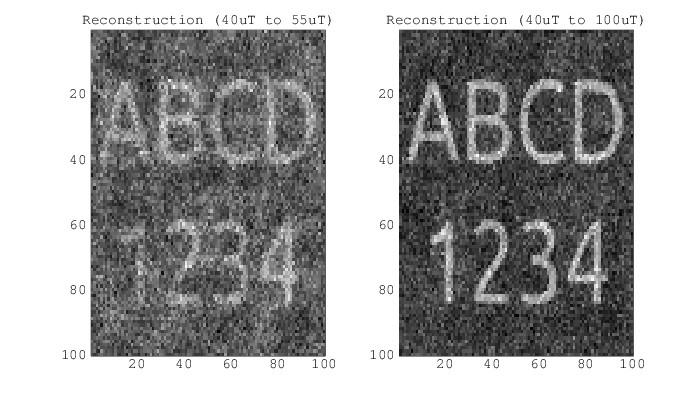
This reconstruction definitely looks a lot better! By 20 measurements we can clearly make out this slice, although it's still a little noisy. For comparison, here are the reconstructions from the two simulations after 20 measurements:

Just for fun, I found two slices online from actual MRIs of produce, and put them into the simulator. The first is an orange with lots of signal, simulated with codes from 40uT to 150uT, out to 20 measurements. The reconstruction looks pretty good! Though the fine structure in the peel and between the orange slices would likely take many more measurements to recover.

And while the test pattern and orange have lots of simulated signal, let's try this apple, whose amplitude is much less intense in most areas. Here we simulate with codes from 40uT to 100uT, but out to 100 measurements (or 5 times longer than the other simulations). This one definitely takes longer to reconstruct, but it does an okay job with the general structure after about 30 measurements, and picks up some of the finer structure and contrasts closer to 90 measurements.

The beginnings of the simulator are starting to take shape, and while these numbers will move around a lot as the simulation becomes more accurate (particularly with the addition of noise, the properties of a radio receiver, and more physically realistic codes that include field orientation), it's encouraging to have and end-to-end system, and begin to get an appreciation for the coded field system along with some very preliminary results.

Thanks for reading!