The image based scheme we used had several processing steps
- Video sequences were shot at either 30 fps or 500 fps. The high-speed sequences were decimated by two in time for analysis. Frames were cropped so that the animal was completely within the frame and filled ½ to ¾ of the frame. A series of video frames were extracted from an AVI file. Typically 100 to 400 frames were used. A short Matlab program reads the AVI file, converts it to a Matlab movie format. The images were downsampled to a resolution of about 120 pixels for analysis.
- The intensity of each frame was normalized because the high-speed camera AGC tended to oscillate a bit. The correction factor used was (SequenceAveragePixelIntensity/FrameAveragePixelIntensity)0.75.
- The motion estimation was based on optical flow computation between frames(3).
A simple gradient optical flow calculation was used to estimate motion. The
video data was arranged as an N by M by T matrix where N is the number of
pixels in the x-direction, M the number in the y direction, and T the number
of video frames. The 3D matrix was smoothed with a 5x5x5 gaussian convolution
kernel with a standard deviation of one pixel. Derivatives in all three directions
were computed using a second-order (centered, 3-point) algorithm. The motion
estimate is based on the notion that pixel intensities only change from frame-to-frame
because of motion. If true, and if
Iis the array of intensities at every point in a frame, andvis the vector velocity of the object seen by the pixel, then
dI/dt = -∇I dot v
or put in words the rate of change of intensity at a point is equal to the spatial gradient of the intensity projected onto the velocity. The dot-product implies that only the projection of v on the gradient can be detected. Put differently, moving at right angles to the gradient causes no intensity change. Solving for the component of v in the direction of the gradient, vg, (perhaps normal to an edge) gives, Vg = -(dI/dt) Del(I)/mag(Del(I))^2 - For each frame, the total pixel motion was estimated by averaging the speeds of all pixels. The "average speed" of a frame was a simple average of the magnitude of v of all the pixels in the frame, as used by Peters, et al on motion studies of the Jacky Dragon. We also defined a "speed surface" (consciously trying to mimic the usefulness of a spectrogram). The speed surface is a 2D plot with the x-axis being frame number, y-axis being pixel speed, and the color proportional to the log of the number of pixels moving at a given speed. In other words, at each frame time we plotted a histogram of pixel speeds.
- Similarity of the various signals was computed by circular cross-correlation. Waveforms being compared were padded to the same length and rotated through frame number. Both average speed waveforms and speed surfaces were analyzed, using 1D correlation for the speed waveforms and 2D correlation (with shifts only along time) for the speed surfaces. For the next stages of the analysis it was more useful to have a measure of dis-similarity, so we used one minus the maximum correlation as a distance measure. Since every signal is correlated with every other signal, the result is a matrix of correlations.
- Given a matrix of distances (of all signals to every other signal) you can compute the strength of the clustering of the signals (perhaps by species) and the entropy of the clustering. The entropy of the clustering is an indication of how well the signals conform to some a-priori clustering scheme.
- The distance matrix can also be used as input to a MDS scheme which attempts to find the best 2D or 3D fit to the distance data. Clusters wihch appear after MDS are determined by a golbal relaxation of distance fits, rather than computing a-priori catagory distances.
The programs
The following matlab programs implemented the various features noted above.
Step 1 above was carried...
 Bruce Land


 Timothy Kanarsky

 Nyeli Kratz
* Note that all the pictures you linked to within the project appear as grey squares, from my end. ;-)