Project Details

Soft oscilloscope

This program:

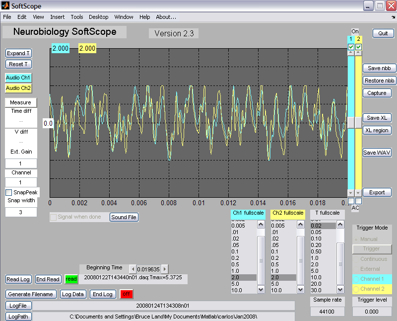
• Simulates the function and appearance of a traditional two-channel oscilloscope. The GUI consists of a simulated oscilloscope, hereafter refered to as the scope.
• Accepts real input from either the Windows sound device, a National Instruments DAQ board or other supported devices. You choose the input device when you start the program.
• Stores data in several formats that other analysis programs can use.
• Recalls stored data to perform analysis on the data

The next two sections explain how to set up the program and how to operate the controls. The program assumes that you have installed the necessary drivers supplied with whatever data aquisition card you are using. The winsound (audio port) drivers are installed with windows, but (for example) the National Instruments interfaces require NIDAQmx 8.3 drivers. This program is cycle and memory hungry. It may not work well on slow machines. The program has only been tested on machines running WindowsXP/SP2.

There are two different ways of setting up the program:

• Program Download version 24 . The Matlab source code version requires the program and requires an licensed, installed version of Matlab R2007a. Be sure that your Matlab 'path' includes the folder where you stored the program. If you are not sure use the SetPath... option in the File menu to investigate.
• The compiled program requires three files (but NOT Matlab):
  • MCRinstaller. You must accept the license on MCRinstaller use before downloading. On older machines, if the MCRinstaller fails with a cryptic error message, you may need to download some C++ stuff from Microsoft. The needed file is vcredist_x86.exe. The .NET stuff from Microsoft may also be required, but not on most machines.
  • An exe which you will double-click to start the program
  • This library file

The scope controls:

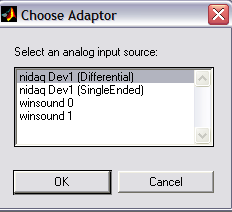
• When you start the program, you must choose an input device from the device dialog box shown below. Some devices have more than one mode (differential/single). Every windows machine will have winsound0. If you cancel out of this dialog, you will get an arror message and the program will quit. Depending on which device you choose, additional controls may appear. For example, choosing the NIDAQ differential device will enable a menu called ADC input range for choosing the full range of the analog input. Choosing a lower range results in limited range (and potential clipping of the wavefrom), but better resolution at low amplitudes.
  
• Channel 1 and 2 controls are color coordinated so that all controls belonging to one channel are the same color (see below for changing the colors). Channel 1 and 2 can be turned off and on by clicking the check-boxes at the upper-right corner of the trace display. Each trace can be set to AC mode which surpresses the average trace value. This is useful for viewing small voltage changes superimposed on a large DC value. AC mode is chosen by clicking the check-boxes in the lower-right corner of the trace display. Traces may be positioned vertically by using the vertical sliders to the right of the display.
• Vertical voltage scale can be set from .001 to 10 volts full scale with the V fullscale control, for each channel separately. Channel 1 scale and Channel 2 scale are shown at the top-left of the plot in appropriately colored boxes.
• Horizontal time scale can be set from .001 second to 30 seconds with the T fullscale control.
• Clicking on the sound file button allows you to load a WAV file, which will be played whenever a trace is complete, if the signal when done checkbox is checked. For large time scales, it is nice to have the program notify you when the trace is complete.
• Trigger source can be set to:
  • Manual, which activates the scope Trigger button. Pressing the Trigger button will cause the scope to acquire one trace. To quit from the program or change the scope time scale, the trigger mode must be Manual.
  • Continuous to acquire data as fast as possible.
  • External to cause the scope to acquire data when an external pulse is applied to analog input 2 with an amplitude greater than the value set in the Trigger Level control.
  • Channel-1 or Channel-2 which triggers the scope when the voltage on the respective channel is equal to the value set in the Trigger Level control.
• Sample rate (samples/second) will snap to 8.0, 11.025, 22.05, or 44.1 kHz for the winsound device and to an arbitrary value for the NIDAQ device. Default is 1000 sample/sec. Sampling a signal at a high frequency uses a lot of memory, but allows you to see higher frequencies in the analog signal. You must sample at a frequency higher than twice the frequency of the input signal, and usually 10 times higher.
• The Expand T control activates a cursor-based drag box. Click on the Expand T control, then click-drag-release in the scope trace display. The part of the waveform you dragged over will expand to fill the display in the horizontal direction. Voltage scaling is not affected. A scrollbar appears so that you can scroll through the entire waveform.
• Audio Ch1 and Ch2 play the traces through the sound card.
• The Measure control activates a cursor-based drag box. Click on the Measure control, then click in the scope trace display. The click sets a zero value. The difference between the zero value and current cursor position is placed in the edit fields below the control. Since each trace can have different gain, you must choose the trace. If you have an external amplifier between you experiment and the computer input, you can set the gain. If you click the Snap Peak box, the measurement will attempt to find a positive peak within Snap Width of the cursor position.
• Save nbb stores the entire data structure of the scope on the disk using a standard dialog box to determine the file name.
• Restore nbb reloads a saved data structure.
• Save XL saves the two voltage traces as an Excel datasheet, with time, trace1 and trace2 as columns.
• XL region saves only the portion of the two voltage traces visible on the screen as an Excel datasheet, with time, trace1 and trace2 as columns.
• Save WAV saves the two traces as a sound file.
• Export causes the entire data structure of the scope to appear in the standard Matlab workspace. You can then access any value from any control:
  • Volage traces are in variables ScopeData.y(:,1) and ScopeData.y(:,2) in units of volts.
  • Time base is in ScopeData.x in units of seconds.
  • Trigger level is in ScopeData.triggerlevel.
  • Sample rate is in ScopeData.Fsin.
  • To view the entire data structure type ScopeData(1) at the Matlab command prompt.
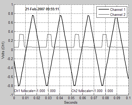
• Capture causes the scope traces to be copied to another window, time stamped, and formated for printing. Once a display has been captured, the standard Matlab print, export, save and edit commands may be used. For instance, you can add a title. Saving the captured image from the file menu allows you to repoen it at a later time. The image below was captured from the traces shown near the top of the page.

• The program can log data directly from the analog input to disk. There are a group of controls for writing and reading a log file. Two wide edit fields near the bottom of the GUI allow you to set the log file name and location for writing. The Generate Filename button will construct a file name for you by generating a time stamp containing the year.month.day.hour.min.sec and a sequence number. The Logfile button allows you to choose a file name, and the Logpath button allows you to choose a folder for the file. You can also type directly into the two edit fields. The Log Data button enables logging. When logging is active a green record indicator is shown, and the log file name and folder are fixed. Each trigger will store data to a different, sequentially numbered, file. Running the scope in Continuous mode will generate one long file. The End log button turns off logging.
• To read a log file, click the Read Log button and open the file. The file name is displayed and a green read indicator is shown. All the scope display controls work, but you cannot get new data. The End Read button restores normal scope function. Note that log files can become huge if you log for along period. One scond of data from the winsound device generates a 0.5 megabyte file. When reading a log file which was recorded for a longer time than the current scope display time, you are able to choose the time (relative to the recording start time) using a small edit/scroll interactor.
• All controls which are channel-specific are color coded to match. Channel 1 controls are blue and channel 2 are yellow. These colors may be changed by editing the program code. If you wish to edit the colors, search for any of the three following statements:
  data.line1color = [.5 1 1];
data.line2color = [1 1 .5];
data.scopecolor = [.4 .4 .4];
  The vector in each statement represents the red, green and blue values for channel 1, channel 2 and the scope background. These vectors can be set to arbitrary values, so long as, each value is between 0 and 1.

Scope Internal Organization (you don't need this to use the scope):

The program is structured as a Matlab function. Persistant data is stored in the UserData area of the figure. The initial execution of the function from the command line initializes a bunch of variables and the GUI, then exits. At that point, the GUI is drawn in the figure window and all the GUI controls are waiting patiently for a user action. Control returns to the main function under three conditions:

• The user triggers a GUI element, and hence a callback function. Each GUI element callback is defined by the following uicontrol parameter: 'CallBack',[data.myname,' action']. The structure element data.myname holds a string which is the name of the file holding the main function. The literal string which follows defines the actual action within the function.
• The DAQ toolbox timers are active and a timer event occurs (to acquire data or produce a pulse). The format for defining a timer action is: set(data.ai, 'TimerAction', {data.myname,'action'}). Where data.ai holds a handle to the analog input device, the litereral TimerAction specifies which action type will be defined and the cell-array {data.myname,'action'}specifies the function and parameter which will be occur when the DAQ timer times out..
• The DAQ toolbox trigger is active and a trigger event occurs (e.g. a voltage passes a threshold). The trigger actions are specified in a similar fashion to timer actions.

Each of the events or callbacks passes a string to the main function which is dispatched by a gigantic case statement to perform an action, perhaps modify the persistant data, then exit. Since the main function is not running most of the time, the Matlab command line stays active.

The DAQ toolbox provides an (almost) hardware-independent, abstract, data acqusition interface to Matlab. Several devices are supported. The current version of this program has been tested with the Winsound device and National Instruments NIDAQ hardware. It turns out that there are some device dependencies so not all hardware will respond correctly. The DAQ toolbox defines analog input objects which have quite complex, and potentially asynchronous, behavior. The usual get/set commands specify DAQ object parameters and read back their state. Debugging the prorgram consisted mostly of figuring out how to set up DAQ objects and their parameters.

Note that it is possible to produce weird concurrent errors if the user happens to trigger a GUI element at just the wrong time. I am still working on this. There are a few sub-functions near the end of the program. One of them displays the scope traces.

Frequency and ISI histogram analysis program

This program:

• Loads data in either nbb format or daq log format. NBB format is included to be compatable with the scope program above. The log format is perferable. There is a specialized version which takes only WAV format.
• Computes a multi-amplitude windowed spike interval histogram from stored data.
• Computes instantaneous frequency (1/ISI) versus time for each amplitude window.
• Exports the frequency vis time plot to an Excel spreadsheet.

Program download (matlab source)

Control description:

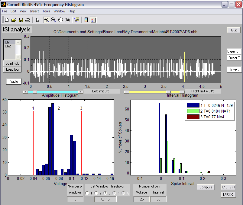
• Raw data (from the aqusition program) is plotted at the top.
  • The only controls which are active initially are the Load buttons. Use the dialog box which pops up to select a file saved from the data aqusition program descibed above, or from another program. Once you have chosen a file the cahnnel dialog box will indicate the channels available. A simulated test file is here. Click the save link as ... option to use this file. The test file contains two simulated units. The small amplitude unit fires about twice as often as the bigger unit. About 200 spikes werre expected for the smaller unit and about 100 for the larger unit. The 7 larger units are summated artifacts.
  • Once data is loaded, you can pick a channel to analyse.
  • Expand T and Reset T buttons enable zooming and panning. Zooming is performed by click-dragging the mouse over the region of interest. Panning is performed by a slider which appears when time is expanded.
  • The Invert button flips the input data.
  • There are two slider controls below the raw data window. The left control sets a beginning analysis cutoff time. The right control sets an ending analysis cutoff time.
  • The Audio button plays the wavefrom through the sound card.
• When you click the Compute button, an amplitude histogram of the spikes is plotted at the lower left and a group of windowed spike interval histograms are plotted at the lower right. A separate histogram is plotted for each active amplitude window.A legend is added to the lower-right plot which gives the averate ISI and number of action potentials in each active amplitude window. In addition, a separate figure is created with the ISI histogram data each time you click this button.
• The number of amplitude windows chosen activates the corresponding number of window threshold buttons. When a window threshold button is selected, the window's lower edge amplitude value may be set. The top edge of the highest window is the maximum amplitude spike detected. The positions of window edges are shown on the amplitude histogram as red lines.
• If you want more resolution in either voltage or interval on either histogram, you can change the number of bins. The Matlab figure zoom control allows you to expand a portion of any plot. The lower-right plot in the example at the top of the page has been zoomed for clarity.
• The 1/ISI vs t button opens a separate window with a plot of 'instantaneous frequency' vs time for each of the windowed spike trains. You have to push the Compute button before you use this feature.
• The 1/ISI-XL button exports the instantaneous frequency vs time data to an Excel spreadsheet. You have to push the Compute button before you use this feature.

Physiological Stimulator

This program uses a analog interface to simulate a physiological pulse stimulator. The stimulator produces a synch pulse on channel 0 and a pulse train on channel 1. Some winsound devices have a 50 Hz highpass characteristic, so pulses longer than about 10 mSec will be distorted when using winsound on those systems. You should check your output with a scope. Output can be single pulses, a pulse train, or a tetanic burst.

Program Download (matlab source version 23)

The stimulator controls.

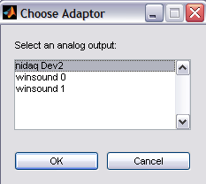
• When you start the program, you must choose an input device from the device dialog box shown below. . Every windows machine will have winsound0. If you cancel out of this dialog, you will get an error message and the program will quit. Depending on which device you choose, the allowed sample rates may be different. Sample rate will snap to 8.0, 11.025, 22.05, or 44.1 kHz for the winsound devices.
  
• Trigger mode can be set to:
  • Single, which activates the Trigger button
  • Continuous to produce pulses at the rate specified by the Repeat Interval control when the Start button is pushed.
• The wavefrom can be set to single pulse, pulse train or tetanic. In tetanic mode, the trigger continuous mode is disabled (in this version).
• All pulse delays and durations are set with a set of edit fields and lef-right arrows. The stimulating waveform is drawn below the controls. The color of each time control corresponds to the color of a line on the drawing.
  
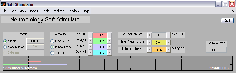
  • In one pulse mode you can set Delay 1 (trigger to pulse) and pulse duration.
  • In pulse train mode you can set Delay 1, Delay 2 (pulse to pulse), Train/Tetanic duration, and pulse duration. The length of each colored line on the drawing corresponds to the setting on the similar-colored control.
    
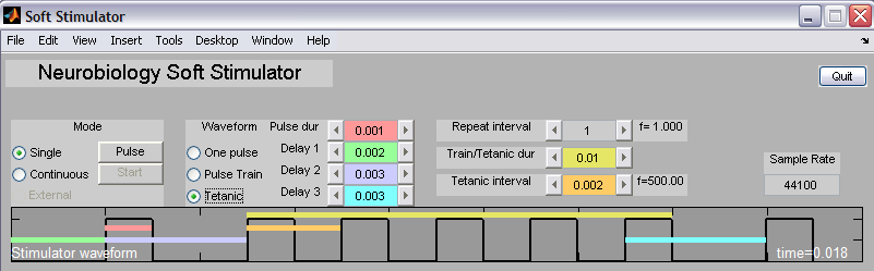
  • In tetanic mode you can set Delay 1, Delay 2 ( first pulse to train), Delay 3 (train to last pulse) and pulse duration. You can also set the tetanic duration which is the length of all the pulses in the train, and the interval which is the spacing of pulses within the train.
  • In all modes, you can set the repeat interval which determines how often the entire stimulus will be produced, if the trigger mode is set to continuous and the start button is pushed.
  • The following image shows the stimulator in tetanic mode. The length of each colored line on the drawing corresponds to the setting on the similar-colored control.

Two Channel Version
There is a two channel version which produces two pulse trains (but no sync pulse). This program uses a analog interface to simulate a physiological pulse stimulator. The stimulator produces a pulse train on channel 0 and a pulse train on channel 1. Some winsound devices have a 50 Hz highpass characteristic, so pulses longer than about 10 mSec will be distorted when using winsound on those systems. You should check your output with a scope. Output is two pulse trains.

Program version 24 (two channel)

The stimulator controls.

• When you start the program, you must choose an input device from the device dialog box shown below. . Every windows machine will have winsound0. If you cancel out of this dialog, you will get an error message and the program will quit. Depending on which device you choose, the allowed sample rates may be different. Sample rate will snap to 8.0, 11.025, 22.05, or 44.1 kHz for the winsound devices.
  
• Trigger mode can be set to:
  • Single, which activates the Trigger button
  • Continuous to produce pulses at the rate specified by the Repeat Interval control when the Start button is pushed.
• All pulse delays and durations are set with a set of edit fields and lef-right arrows. The stimulating waveform is drawn below the controls. The color of each time control corresponds to the color of a line on the drawing.
  
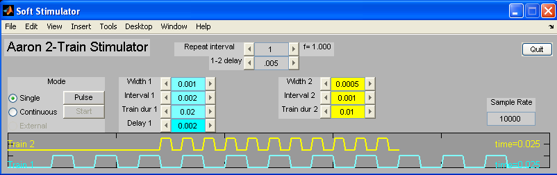
  • The pulse width, pulse interval, and train duration can be set for each train.
  • The delay of train 1 can be set, as can the difference between the start times of the two trains. The difference can be positive or negative (train 2 starts before train 1). Neither trace can start at negative time, however. Zero time is the left edge of the waveform panel.
  • You can set the repeat interval which determines how often the entire stimulus will be produced, if the trigger mode is set to continuous and the start button is pushed.
  • The following image shows the stimulator set to produce two pulse trains of unequal length, pulse duration and spacing.

Stimulus Editor and WAV player

This program:

• Presents a GUI which allows a user to edit a waveform by dragging control points.
• The control point positions are interpolated to a user-selectable sample frequency.
• Interpolation method is selectable
• The number of control points and theduration and amplitude ranges are selectable
• For precision, there is a selectable snap-to-grid function in either time or amplitude.
• Exports the waveform in WAV, text, or matlab format.
• (As a matlab tidbit, this program uses a better scheme for defining window button functions)

Program download (matlab source)

Control description:

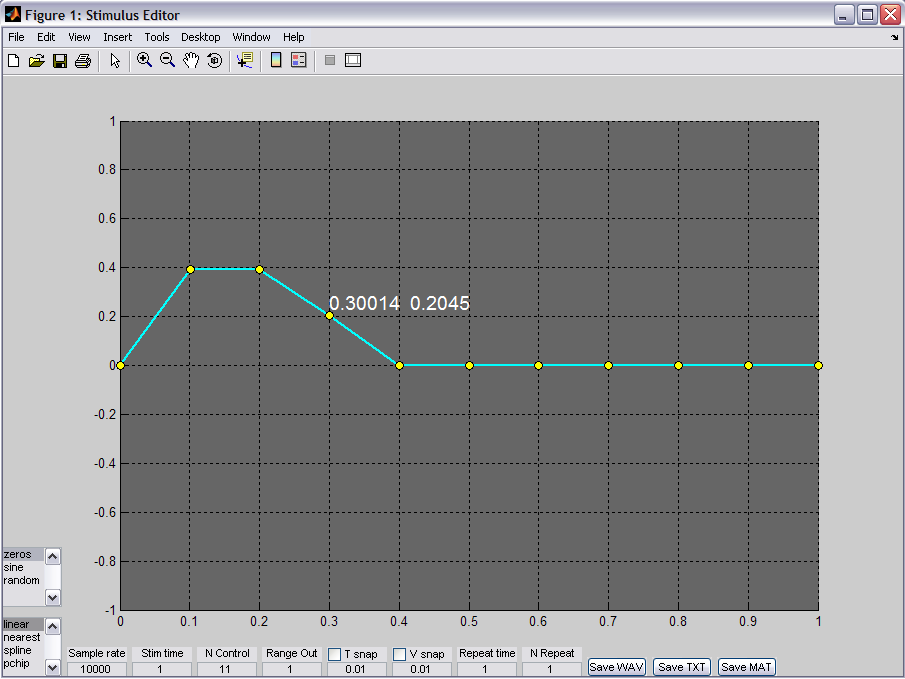
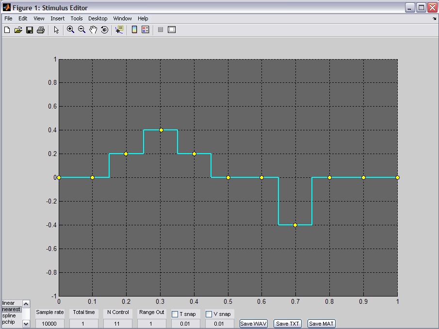
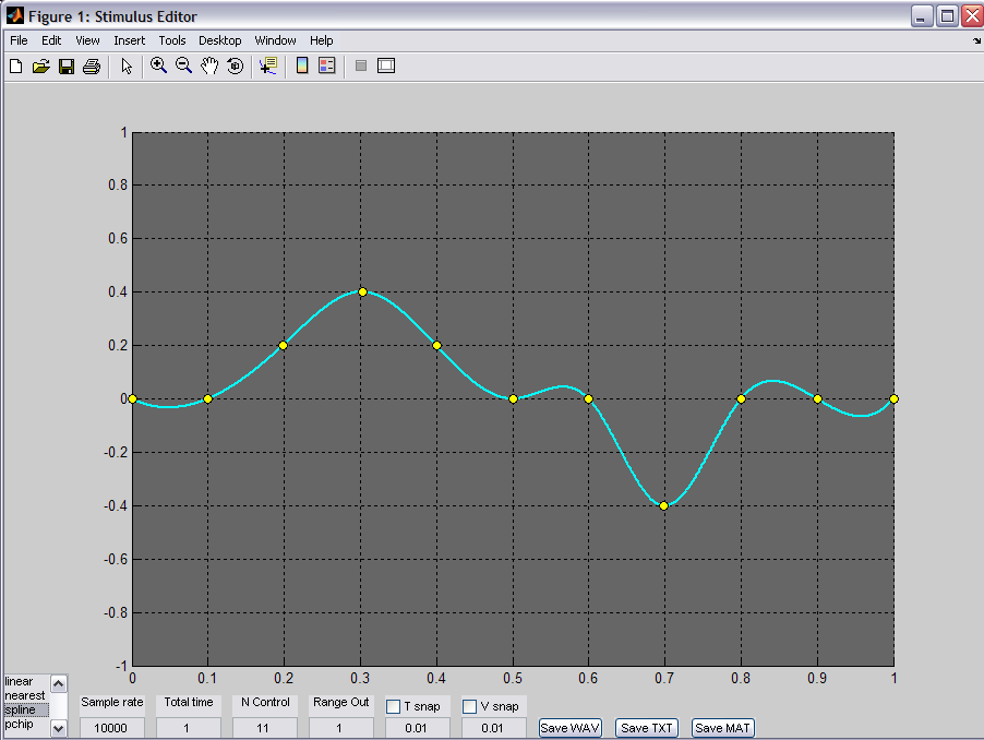
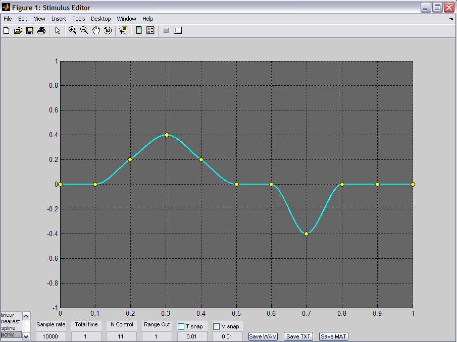
• The list interactor on the lower-left chooses between linear, nearest neighbor (squarewave), cubic-spline, and pchip (modified spline) interpolation. Examples of the four methods are shown below using the same control points.
  
• The list interactor just above the lower-left corner sets the initial state of the control points. You can choose to start with zeros, sinewave, or uniform random control points. Choosing sinewave, with spline interpolation, produces a low-distortion sine wave. Choosing random produces a bandlimited random signal.
• Sample rate chooses the number of samples/second in the output waveform.
• Total time chooses the horizontal time scale in seconds.
• N control chooses the number of control points.
• Range out chooses the vertical voltage scale. If you save as a WAV, the range cannot be greater then 1.0.
• T snap and V snap turn on and set the increment for a snap grid to make alignment easier.
• Repeat Time sets the time between repetitions of the displayed wave.
• N Repeats sets the total number of times the displayed wave will be concatenated with itself. A large N can use a lot of memory fast!
• The three Save buttons save the waveform as a single channel WAV file, as a two column (time,voltage) text file, or as a two column (time,voltage) mat file.
• Clicking on any control point displays the coordinates of the point. The point can then be dragged to a new location.

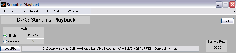
A small utility program plays back WAV files produced by the stimulus editor.

Program download (matlab source)

To use this program

• The program first prompts for the interface device as shown below.
  
• Click the WavFile button to pick a file.
• Once you have loaded the file you can play the WAV once by clicking the PlayOnce button
• You can loop the WAV file by choosing the Continuous option and clicking Start.