AVR
AVR-
SunLeaf to Cloud Communication: Connecting to Thingspeak
08/16/2016 at 14:35 • 0 commentsIntroduction
This is a short log demonstrating how this is done with the SunLeaf module. We have end to end communication between the SunLeaf and the cloud. Right now this is a demonstration of feasibility in that this processor stack (ESP8266 and STMF446RE) can successfully post data to a cloud based server. We all know it will work in theory but it is always nice to prove things work in practice too. This is the purpose of this log.
Code algorithm
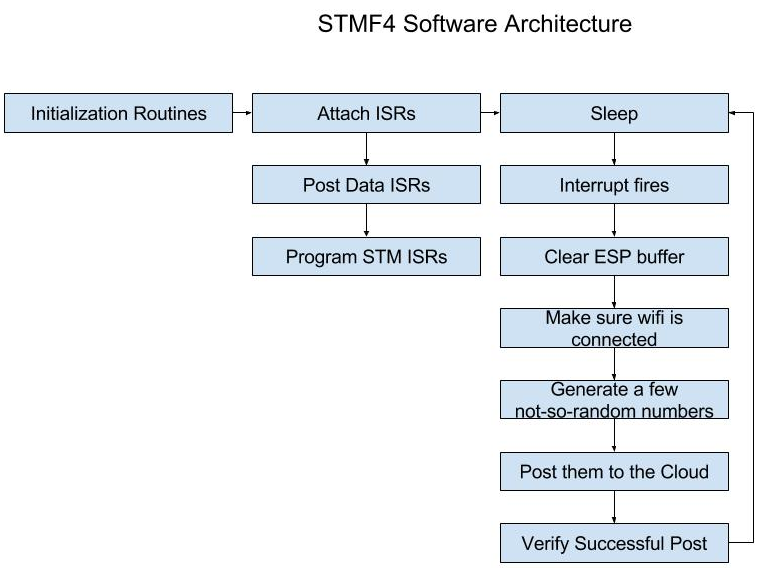
Below is an overview of what the code does. There are three high level tasks. First we initialize all the drivers and the SLIP protocol. Then we attach the callbacks. Lastly we put the STM into sleep mode. In sleep mode all power is cut to the sensors and the ESP is also put into sleep mode. When an interrupt is fired then it wakes up and preforms the data post. The programming interrupt will be an external pin change.

The STM code is here. We'll migrate it to Git shortly.
https://developer.mbed.org/users/ShaneKirkbride/code/STM-Client/ .
This will work with the ESP-Link software as-is:
https://github.com/jeelabs/esp-link
The SunLeaf ESP-Link fork is going to have quite a few changes but use this repo for now.
Data Output Overview
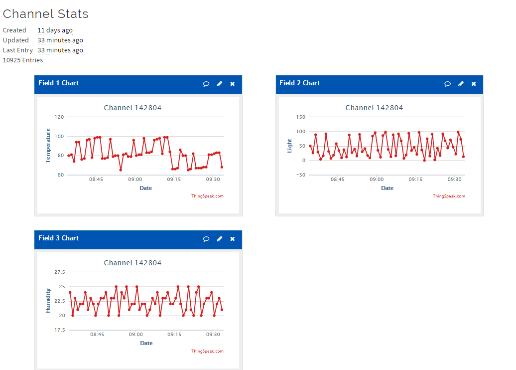
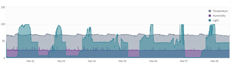
We have not yet connected the sensors and incorporated the sensor drivers. That will be for another post. The data we are uploading is very-psudo-random data generated by the STM not-so-random number generator. Right now we are simulating temperature, light and humidity data. After we build the Kalman filter then we'll upload the estimates as well. You can see the raw data and how not very random the STM number generator is. It is better than looking at the same value each post. Currently we post once per minute. In the future this will be pre-set to once every 10 mins and we will give the user the ability to change the frequency as needed.
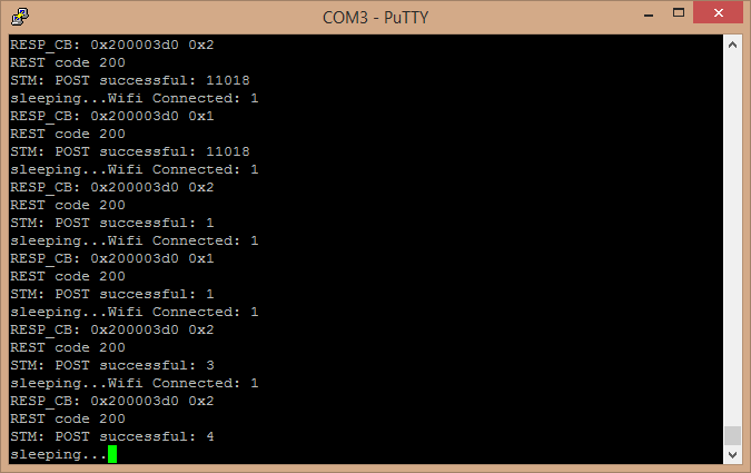
Here is the output of the serial debug channel on the STM.
This output shows the state the ESP and the SLIP connection are in. It also shows if the wifi is connected and if the post is successful.
SunLeaf Thingspeak Channels
We will update this section as we create more channels. Later in the project life we'll migrate to a Viviaplanet cloud server but this shows proof of concept until that time.
-
ESP to STM32 Communication: SLIP Interface
07/26/2016 at 12:23 • 1 commentIntroduction
In the last post about communication we discussed what it took to build up the ESP tool chain as well as the STM32 Toolchain. We loaded the esp-link interface on to the esp and a simple serial communication program onto the STM32 and had the two micro-controllers communicate. It was amazing but for the Sunleaf team sending data between micro-controllers just wasn't enough. We are building a next generation internet of things device. This means it has to work with a cloud system. This also means we need to be able to do basic REST commands. If you need to know more about REST commands I added a link here.
The esp-link supports micro-controller REST Commands but only though a Serial Line Internet Protocol SLIP interface. This was a surprise. Initially we were planning on using simple AT commands to 'GET' and 'POST' data. But there are a few issues with this. The basic serial communication protocol is error prone. Even with some nice libraries that do error checking we still experienced a few errors in the communication. It is also slower. We really though the right way to build this up is to add a SLIP interface to the STM32 so we can communicate with the esp-link and the rest of the internet reliably and quickly. In this log we first discuss what SLIP is. Then we'll cover the port we are using for the STM and give a working example.
SLIP: What is it, really?
When I first realized that I needed a SLIP interface I was hopeful. The STM32F446RE is a fairly common chip. There had to be someone working on an open source version that I could use. I couldn't find one. There are a lot of closed source versions available, if you have between $10K-$30K to drop on a license... But if that's you then you probably aren't reading this now. This definitely isn't us. So we decided we needed to build our own. To do this we needed to learn a little more about SLIP, why it exists and why is it used?
The SLIP protocol consists of commands with binary arguments sent from the attached the STM32 to the esp8266. The ESP8266 then performs the command and responds back. The responses back use a callback address in the attached STM-Client code. For example the command sent by the STM32 contains a callback address and the response from the esp8266 starts with that callback address. This enables asynchronous communication where esp-link can notify the STM32 when requests complete or when other actions happen, such as wifi connectivity status changes or RSSI Values...
However, there is no true internet standard for Serial Line IP. There is a good deal of work done on this still. It is intended to work as a point-to-point serial connection for TCP/IP connections.
SLIP is commonly used on dedicated serial links but has been replaced on many CPUs with PPP. For embedded systems like the STM32F+ESP8266 system it works well. It is also nice because I don't have to post my SSID and wifi password wit this configuration. This is because SLIP allows mixes of hosts and routes to communicate with one another (host-host, host-router and router- router are all common SLIP network configurations).
Basically it is a simple two layer protocol providing basic IP framing. Here is a diagram of how the protocol is supposed to work:
Here is a summary of SLIP:
- Breaks an IP datagram into bytes.
- Send the END character (value “192”) after the first and last byte of the datagram;
- If any byte to be sent in the datagram is “192”, replace it with “219 220”.
- If any byte to be sent is “219”, replace it with “219 221”
Kinda nifty? Well, not really. It is very old but for an embedded system to post reliable REST requests it is top-notch. Next we talk about how it is implemented in the STM32F446RE Board.
SLIP for the STM32: STM-Client Overview
As we discussed we've loaded a sun leaf version of the esp-link software onto the ESP. Here is where the source is kept: https://github.com/jeelabs/esp-link. Now, versions of esp-link use the SLIP protocol over the serial link to support simple outbound HTTP REST requests and an MQTT client. There are examples of these libraries for REST and MQTT libraries as well as demo sketches in the el-client repository. These only work on Arduino boards and I think a few NXP boards. If you want to use a real micro-controller you'll have to port some of this to C. Which is what I did...so I guess you don't have to any more...
The homepage for the mbed repository: https://developer.mbed.org/users/ShaneKirkbride/code/STM-Client/
Again keeping in mind that is is largely ported from the EL-Client repository here are some highlights about how this port works. First there are two serial objects that the client requires: Serial and DebugSerial. This is extreamly helpful because you are essentially blind to what is going on inside the STM32 once the program kicks off unless you use the debugSerial object. In the El-Client repo there is no true main.cpp for the rest example. This is because the program is intended for the Arduino. So the first thing we did was make our own. It was a very similiar example. The main difference is that the STM32 (or maybe the mbed API...) dosen't support asynchronous communication. There are a lot of stream objects in the Arduino code that don't port correctly to C.
This is fairly easy to overcome by Arduino the serial objects in main and changing the stream* datatype classes to serial* datatypes. This was really the biggest catch. Once I figured this out the only other trick was to reset the ESP8266. A lot of research went into figuring out how to do this correctly. I almost ported a LWIP library but found the STM-Client to work better.
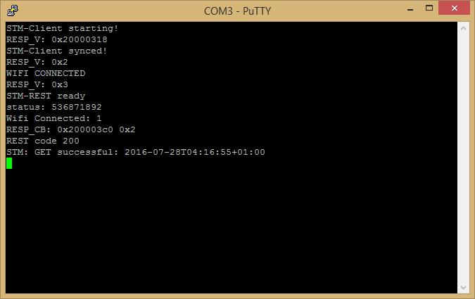
Here is a screen shot of the system sending a 'get' request to www.timeapi.org.
I used putty...but you can use any serial output. This text is all through the serial debug port.There is also a 'post' example that is commented out in the code for posttestserver.com. This also works but I'm working on this to get it talking to vivaplanet right now so it has limited functionality.
There are a few more firmware goals we are going to address in the next two months. The first will be posting to a cloud based server: vivaplanet. Posting to something like an Azure cloud service is non-trival for a platform but I'm confident it can be done. The second is OTA programming the STM32. This is also non-trival and may require a hardware change to the rev 2 board. Lastly, I need to get the Kalman filter engine working. If we're lucky we'll get to all of these topics before October. We also need a rev 2 board and a rugged mechanical housing but that will also be coming soon to a log entry near you.
-
Hardware Assembly
07/02/2016 at 19:05 • 0 commentsSo the last few updates on the SunLeaf have been about sensing and software. Last time we touched on the hardware was when the boards and components were ordered. Quite a bit had developed since then. Since then a single SunLeaf prototyep has been assembled and ready for testing, after testing the next two from the batch will be assembled/populated.
SunLeaf Prototype PCBs as they arrived in the Mail.
Some of the Components and Solder Pastes.
For the sake of cost and time of this project, the first SunLeaf was assembled by hand using a reflow hot air station and standard soldering iron. All the assembly was conducted under a stereo microscope, this was very helpful for soldering 0402s in close proximity to connectors and ICs. The scope as also essential in lining up the pins on the STM32 F4's TQFP package. Each component was placed one at a time in order as they appear in the BOM, ICs were all placed last. The prototype was soldered using lead-free low temp solder paste to parts can be easily removed, also some components like crystals can be sensitive to heat. All the paste and flux was applied to the board by hand, since I lacked an air compressor for my paste dispenser. Now the board has parts on the top and bottom, I though this was going to pose an issue but it did not, I simply populated the top side and when it was complete I did the bottom side, just flipping the board in the stick vise.
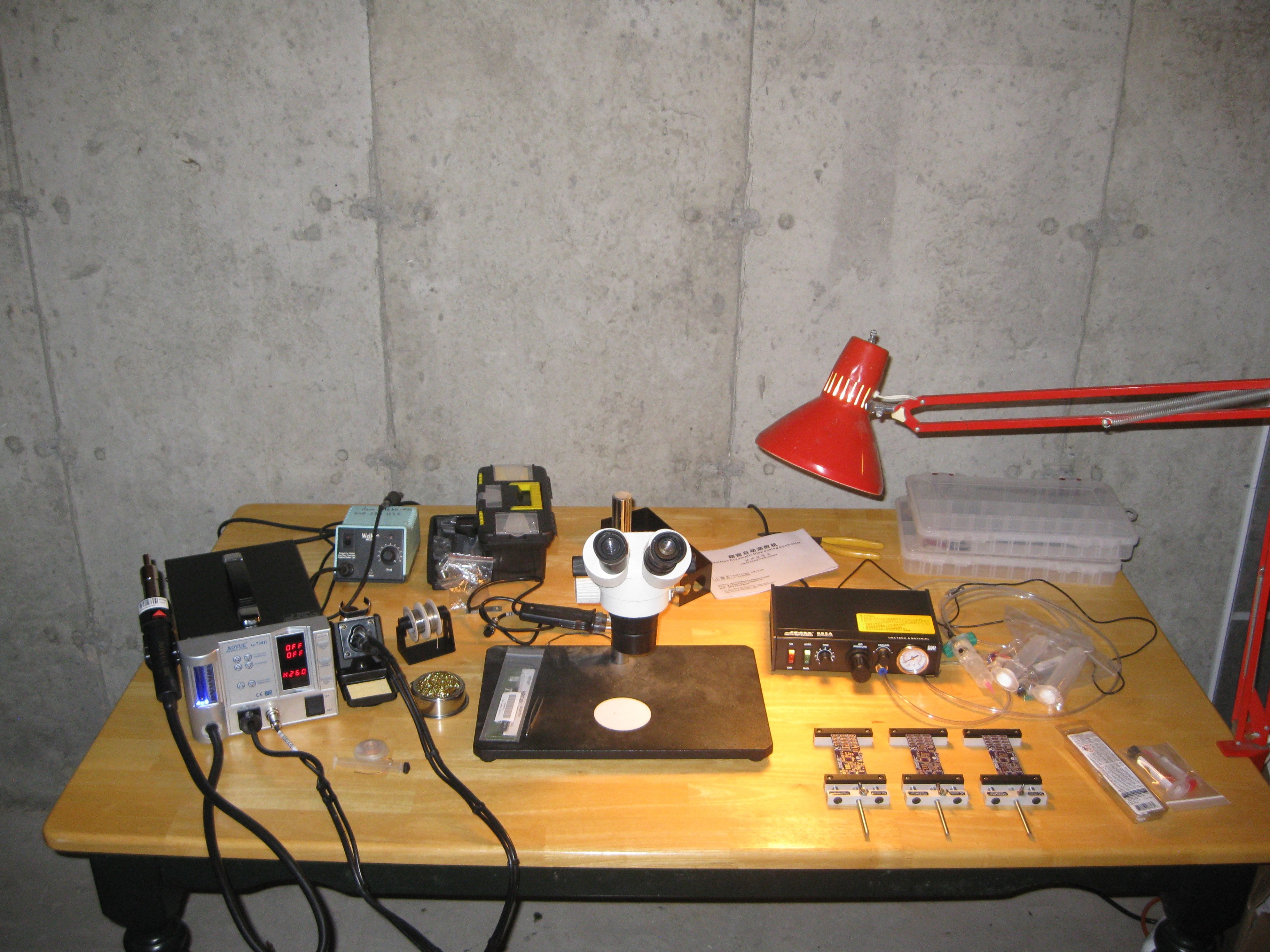
Quick look at the soldering setup/Lab
Notes the 3 Stickvise's, having three of them is actually a lot handier than I thought :)Now for the moment you've been waiting for:
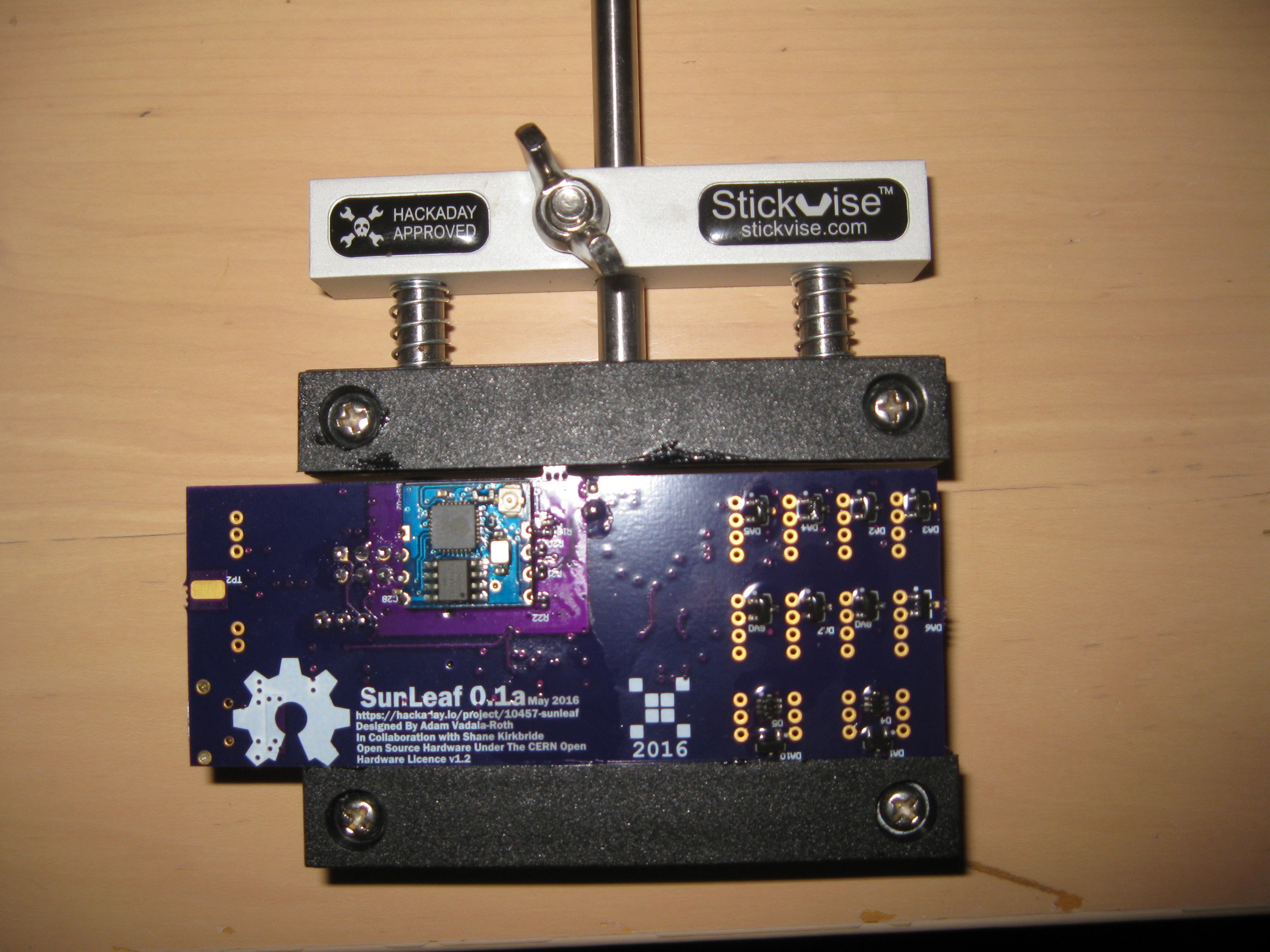
Bottom ViewMuch apologies for the dirty PCB covered in flux lol. There you have it though, this is the first populated SunLeaf, now you will notice some components are missing. In my experience I like to solder throughhole components like the connectors last, if they are soldered on earlier in the process then the plastic tends to get burned by the hot air. You will also notice that the solar charging section of the PCB has been left unpopulated. There is a a flaw in the footprint of the battery charging IC, the pins were flipped, oppisite of the datasheet, its an honest mistake but it makes that section of the board non functional. In the second revisions this error will be fixed as will any others found during testing. Lucky enough the SunLeaf is setup to accept power for its onboard regulator from either the USB port or the solar panel/battery so for the sake of the project an completing all the software we are still in business. So what's next? Next I have to give the PCB a thorough cleaning to remove excess flux and solderpaste particles, this is done to prevent shorts or malfunctions in the device that could be caused by an unclean assembly. So with that said stay tuned because testing is the next step in the hardware process, hopefully we will have some functioning hardware in the days to come, stay tuned!
-
Embedded Sensor Fusion: Part 3 The simulation
06/29/2016 at 18:42 • 0 commentsIntroduction
In this section we're going to go over the performance of the IMM-KF. Basically this will involve walking through the Matlab code that I used. First I'm going to discus how I constructed the final system. Then I'm going to highlight some of the key calculations within the code. After that we'll look at the simulation results. Finally I'll post the entire set of code and the data I used for you to test (and maybe improve). A lot of this code orginated from Yaakov Barshalom's website. He wrote a really cool book called "Estimation with Applications to Tracking and Navigation".
Simulation walk through
The simulation algorithm has 5 basic parts. The system set up, loading the measurement data, running the Kalman filter and then the interaction between the models. The system set up consists of building the state space and initializing all the noise and other variables. This is probably the most important step because if you get it wrong nothing will work. It is also easy to get kind of right but not perfect.
The system set up
Earlier we determined there were two distinct models that this data was in. The first was the NCP model and the second was the NCV model. These are both corresponding modes. In addition to the states we'll also need to keep track of the probability of the system being in a given mode.
Sensor Fusion: Building the state-space
There are two ways to run this IMM-KF. The first approach would be to run each measurement though the algorithm for an independent estimate. This would be an OK way to estimate the problem but it is not really fusing any sensors nor does it allow us to couple the dynamics of the system and it would in the end result in a less accurate estimate of the state of the flora. One more item to note here is that these state space models can be improved. These are initial best guesses but after time the sensor dynamics can be added into these models. If we were to fuse the states of each sensor together we'd get something that looks like this:
Mode 1 (NCV)
So this the discrete time state space equation for the nearly constant velocity model. It is taking all of the sensor measurements into account as well as the rate they are changing. This model would ideally be used during a transitional state in temperature, time or humidity.
Here is what the code looks like:
% Set up model 1 for mode 1: NCV model, 3 sensor measurements dimensional, T=5
% Start with discrete-time (continuous time is for wimps)
T = 1;
A1 = [ 1 T 0 0 0 0 0;...
       0 1 0 0 0 0 0;...
       0 0 1 T 0 0 0;...
       0 0 0 1 0 0 0;...
       0 0 0 0 1 T 0;...
       0 0 0 0 0 1 0;...
       0 0 0 0 0 0 0];

Bd1 = [.5*T^2 0 0;...
       T      0 0;...
       0 .5*T^2 0;...
       0 T      0;...
       0 0 .5*T^2;...
       0 0 T     ;...
       0 0 0     ];
B1=Bd1;
C1 = [1 0 0 0 0 0 0;...
      0 0 1 0 0 0 0;...
      0 0 0 0 1 0 0];
Mode 2 (NCP)
So this the discrete time state space equation for the nearly constant position model. It is taking all of the sensor measurements into account. We presume a constant position but the matrices need to be the right size for the multiplication operations so I just 'zero' out the velocity channels in this model. This model would ideally be used during a steady state in temperature, time or humidity.
Here is what the code looks like:Ac = zeros(7); Bc = [1 0 0;... 0 0 0;... 0 1 0;... 0 0 0; 0 0 1;... 0 0 0;... 0 0 0]; [A2 B2] = c2d(Ac,Bc,T); C2 = [1 0 0 0 0 0 0;... 0 0 1 0 0 0 0;... 0 0 0 0 1 0 0];Estimating the noise
Estimating the noise initializations values is complicated. There is a lot of mathematics in the code showing how to do this. But in the end the best way is to just run the data and look at the process and sensor noise at the end of the simulation and use these values. It gives good results to start with.
Loading the measurement data
This is the most straight forward part of the simulation. The data was uploaded to the vivaplanet cloud in JSON format. There is a nice little matlab package that will sort out the JSON data in to cells. So I use this data for my true values of my system. We know they are the actual true values but they are the measured values and the best estimate we have before we compare them with the state spaces.
Here is what the code looks like for this. Notice I allocated those matrices I knew the static size of.
%% Generate the true system data
xtrue = zeros([7,dataLength+1]);
z = zeros(3,dataLength);
t=zeros([1,dataLength+1]);

for k = 1:length(data.Data),
    xtrue(:,k) = [str2num(data.Data{1,k}.Sensor.T) xtrue(2,k) str2num(data.Data{1,k}.Sensor.L) xtrue(4,k) str2num(data.Data{1,k}.Sensor.H) xtrue(6,k) xtrue(7,k)];
    xtrue(:,k+1) = A1*xtrue(:,k);
    z(:,k) = C1*xtrue(:,k+1);

    monthStr = data.Data{1,k}.Sensor.Time(5:7);
    monthNum = find(ismember(MonthNames, monthStr));
    dayNum = str2double(data.Data{1,k}.Sensor.Time(9:11));
    yearNum = str2double(data.Data{1,k}.Sensor.Time(12:16));
    hourNum = str2double(data.Data{1,k}.Sensor.Time(17:18));
    minNum = str2double(data.Data{1,k}.Sensor.Time(20:21));
    secondNum = str2double(data.Data{1,k}.Sensor.Time(23:24));

    t(k) = datenum(yearNum,monthNum,dayNum,hourNum,minNum,secondNum);

end
So now we have some fancy sensor-fused models and some nice real world data and some not-so nice real world data. All we need to do now is implement the mathematics for the IMM-KF.
Initializing and interacting the data
When we start the IMM-KF we need to make sure there are a few calculations done up from.
The first is calculating the the conditional probability "mu" of being in NCV or NCP mode at a given time:
Where m is the mode at any given time. First we calculate cbar:This is the code for this. It is cool because it can be done as a matrix multiplication and results in a vector:% 1) Compute cbar = sum(p(i,j)*mu(i,k-1)) cbar = immData.txprob'*immState.mode;
Then compute the conditional probability or "mu":
% 2) Compute mu(i|j,k-1) = 1/cbar * p(i,j)*mu(i,k-1)
modeij = immData.txprob.*(immState.mode*(cbar.^(-1))');
modeij(isnan(modeij)) = 0; % take care of impossible final states
now that mu is calculated we can blend the state outputs from the last step according the the probably of their current contribution to this state. The equation for this is as follows:
this is what the code looks like:% 3) Compute xhat(mod) x0 = immState.X*modeij;For the last step we calculate the co-variance matrix:
There are two main terms here. The first term is the mixture of the prior covariances, and the second term is due to the “spread of the means” of the individual filters. Yeah...you need a for loop for this guy:
% 4) Compute Sigma(mod).
Sx0 = immState.SX; Sx1 = immState.SX; % reserve space for Sx0,Sx1
for j = 1:modes,
     xk1 = immState.X(:,j); Sx = xk1*xk1'; Sx0(:,j) = Sx(:);
    xk1 = x0(:,j); Sx = xk1*xk1'; Sx1(:,j) = Sx(:);
end
Sx0 = (immState.SX + Sx0)*modeij - Sx1; % verified
at the end of this step you have the covariance matrix, state estate and mode probabilities so now we can move on to the Kalman filter steps.
running the Kalman filter
Now we crank this information through the Kalman filter. You could probably run this loop as a stand alone filter if you wanted. I'm not going to talk through the matlab syntax there are a lot of other good places online to go for this.
First we set up all of the estimates and covariances:
% 0) Set up variables for this filter
xhat = x0(:,j); Sx(:) = Sx0(:,j);
A = immData.A(:,:,j); B = immData.B(:,:,j);
C = immData.C(:,:,j); D = immData.D(:,:,j);
Sw = immData.Sw(:,:,j); Sv = immData.Sv(:,:,j);
Then we calculate the state estimate time update. Where the predicted state is the standard state space equation:% 1) State estimate time update xhat = A*xhat + B*u;Then we preform the predicted covariance time update:% 2) State covariance time update Sx = A*Sx*A' + Sw;Then calculate the output
% 3) Output estimate
zhat = C*xhat + D*u;
Now calculate the gain matrix:% 4) Filter gain matrix Py = (C*Sx*C'+Sv); L = Sx*C'/Py;Next we do the state estimate measurement update:
% 5) State estimate measurement update
immState.X(:,j) = xhat + L*(z-zhat);
Last, the state covariance is updated:% 6) State covariance measurement update Sx = Sx - L*Py*L';After this we calculate the likelyhood of the system is being in a given state:Lambda(j) = max(1e-9,exp(-0.5 * ((max(z-zhat))/max(max(Py))))/sqrt(2*pi*max(max(Py)))); % much faster than normpdfThe kalman filter will need to iterate these steps for each mode. After each mode is calculated we combine the data.
Combining the data
First we calculate the posteriori probability of being in mode NCV is at time k
% Combination step
% 1) Compute PMF of being in mode j: mu(j,k)
immState.mode = Lambda.*cbar;
immState.mode = immState.mode/sum(immState.mode);
then the state estimate is calculated. A mix of the individual filter estimates is the filter output. The value indicates the likelihood of the target being in NCV or NCP mode.here's the matlab code for this math
% 2) Compute composite state estimate
immState.xhat = immState.X*immState.mode;
now we calculate the the covariance mode output:
and here's the matlab code for this math:% 3) Compute composite covariance estimate modeSx = immState.SX; for j=1:modes xk1=immState.X(:,j)-immState.xhat; Sx=xk1*xk1'; modeSx(:,j)=Sx(:); end immState.SigmaX(:) = (immState.SX+modeSx)*immState.mode;There is also some auxiliary driver code in the files that work to drive some of these main functions. Feel free to ask about them in the comments but I'm not going to go over it here. Instead I want to get to the simulation results and show how this code is working.Simulation Results
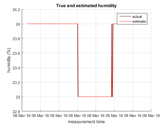
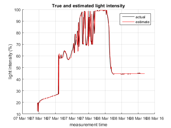
For the simulation I use two data sets. On one data set the humidity sensor is having an electrical issue and on the other data set the humidity sensor is fine. These data sets are about 4300 samples and are to large to show the entire simulation and have it be helpful. Instead I've zoomed into samples 3930-4230. The x-axis shows the date the measurement was taken but the time is buried in the code. This selection shows a few constant position states as well as some constant velocity states. It also shows how some of the system noise is handled when the sensors are fused together. It is a negative to using the raw estimate but since the state and noise info will be sent to the cloud it can be cleaned up post processing. The important information is in the state estimate more than the actual estimated sensor estimates. The code outputs some other data as well but the images below show the important parts of the performance of the algorithm.
Data set 1: good data (set 3)
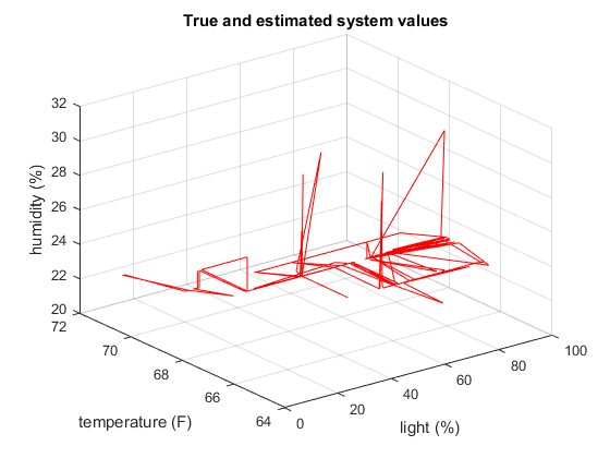
Above is the entire system plotted on a 3D graph to give an idea of the big picture of what is being estimated
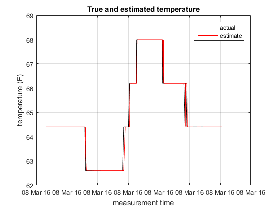
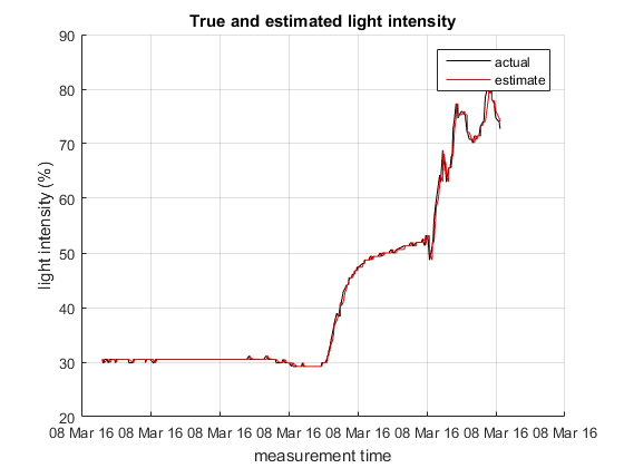
The graph above shows the temperature sensor measurement and the estimate. The estimate is following the measure closely here.The graph above shows the light sensor measurement and the estimate. The estimate is following the measure closely here.
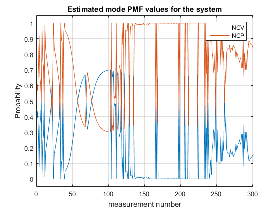
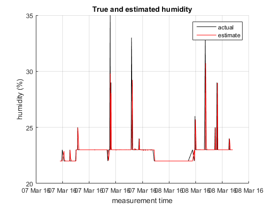
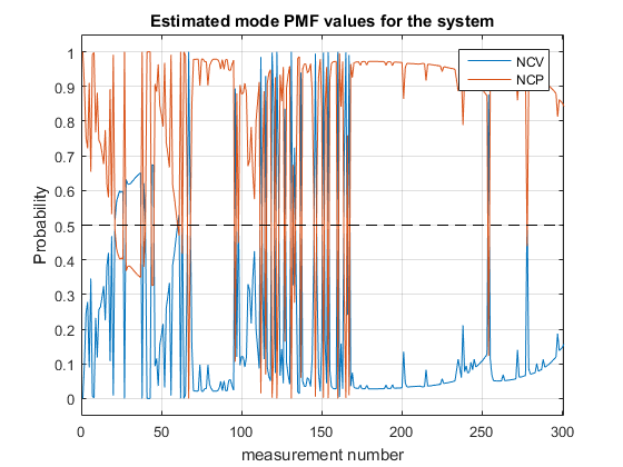
The graph above shows the humidity sensor measurement and the estimate. The estimate is following the measure closely here.The graph above shows the probability the system is in a given mode. You can see this graph working when the system is not changing it tends to be in NCP mode and when the system does start to change it is in NCV mode more. One aspect of coupling these sensors is that the mode needs to account for all 3 sensor changes at the same time. You can see this occurring with this graph.Data set 2: noisy humidity sensor (set 1)
Above is the entire system plotted on a 3D graph to give an idea of the big picture of what is being estimated. This is clearly a more noisy system.
The graph above shows the humidity sensor measurement and the estimate. The filter does not believe this noisy data as much so the actual and the estimates are different. In this case the estimate of the humidity is more accurate than the actual measurement.
The graph above shows the light sensor measurement and the estimate. This measurement is also more noisy. The filter still follows the data pretty well.The graph above shows the temperature sensor measurement and the estimate. The estimate is following the measure closely here.
The graph above shows the probability the system is in a given mode. You can see this graph working when the system is not changing it tends to be in NCP mode and when the system does start to change it is in NCV mode more. One aspect of coupling these sensors is that the mode needs to account for all 3 sensor changes at the same time. In the more noisy system the modes are likely to change more. There is also less overall certianty of the actual mode.Wrap up
I've uploaded the files for this simulation to the site. I'll put the IMM-KF engine in C in the mBed repository for the STM32. This code won't be ready until late July as I'm still working out some of the embedded infrastructure for this entire design. So there will be a part 4: implementation but this won't be until later in the year.
-
Embedded Sensor Fusion: Part 2 the algorithm
06/22/2016 at 18:56 • 0 commentsIntroduction
In the last post we saw there were two types of models for the system: NCP and NCV. The light measurements were modeled as an NCV type system while the temperature and humidity measurements were modeled as an NCP type system. We have some values for these systems and a brief description on how we came up with the first guess values. In this section we discuss the algorithm we use to estimate the measurements from the sensors. I thought about this a little more and I think the temperature and humidity measurements could also be modeled as an NCV type system and the light measurements, at times could look like an NCP type system. There are a few different tools/filters/algorithms to estimate measurements. I'm going to use a Kalman filter for this this estimation. Furthermore I'm going to use an Interacting Multiple Model Kalman Filter (IMM-KF). The reason that I'm using one of these filters is because:
- The measurements that we wish to track has two significantly distinct modes of operation.
- The measurements act like NCV for a period of time, then NCP for another period of time.
The IMM-KF operates multiple Kalman filters in parallel, and systematically mixes state and covariance calcuations each filter to make a composite state estimate and covariance. It is nifty. A much better source than myself for this type of algorithm can be found here:
Mazor, E., Averbuch, A., Bar-Shalom, Y., and Dayan, J., “Interacting multiple model methods
in target tracking: A survey,” IEEE Trans. Aerospace and Electronic Systems, 34(1), Jan. 1998, 103–123.
Before I get into this too much more I want to acknowledge Dr. Greg Plett at UCCS for a lot of these ideas as well and the great notes that he provides to his classes.
So what does this IMM-KF ultimately do? It calculates a probability mass function for the tendency for the system to be operating within a given state. This means that we need to give an probably of transition matrix for each mode. So in mathematical terms specific to the project:
Where mk is the mode at time k. Before we get too deep into the IMM-KF lets go over the Kalman filter.The Kalman Filter
I've linked the Wikipedia page above to Kalman filters for a deeper understanding but before I move on to how the IMM algorithm makes an estimation I need to at least go over the Kalman filter algorithm at a high level. This filter makes a three key assumptions about the system.
- We assume that the system dynamics are linear and that it has a PDF that is Gaussian in nature. Most real world systems are not perfectly linear but when I look at the data from our initial measurements I think there are many features of a linear system + noise.
- The system can be modeled in the state space form:
3. We also assume that the noise processes wk and vk are random mutually uncorrelated white Gaussian with zero mean and covarance matrices in the follow in format:
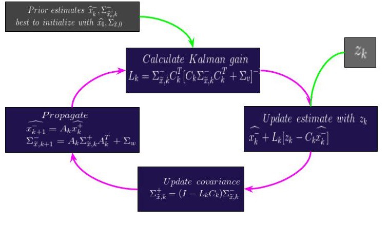
and We make these assumptions knowing real systems are never truly linear but it is these algorithms still work really well. It may also comfort you (it comforts me at least) to know that the Kalman filter is the most optimal minimum-mean-squared-error and maximum-likelihood estimator filter you can use for a linear system-but good luck proving this to yourself. So based on these assumptions we can implement the Kalman filter. The Kalman filter calculation can be broken down in to six (easy?) steps. Only an description is given here of what is going on with the key equations. You'll be able to see the mathematics at work in the code, hopefully:- State estimate time update
This step calculates the current system state using past measurement information. Typically this means the system will need to be 'initialized' and measured with out any estimation before the Kalman filter is started.
2. Error co-variance time update:
This step calculates a the error covariance estimation of the state prediction. The most recent covariance estimate is calculated then propagated forward in time.
3. Estimate system output
This is the most important step in the Kalman filter estimation process because it generates the real world information that is useful. The result of this step is the best estimate the output given the output equation of the system model, and our best estimate of the current system state.
4. Estimate the Kalman gain matrix
The computation of the gain matrix is the most defining aspect of Kalman filtering and distinguishes the algorithm from other estimation methods. The purpose for calculating covariance matrices is to be able to update the gain matrix. The gain matrix is time-varying. This means it adapts to give the best update to the state estimate based on present conditions.
5. State estimate measurement update
The output estimate is what we expect the measurement to be, based on our state estimate at the moment. So we take the actual measurement and determine what is unexpected or new in the measurement. This is called the innovation. It can be due to an inaccurate system model, state error, or sensor noise. Or maybe all of these. This new information updates the state, but it is weighted according to the value of the information it contains.
6. Error covariance measurement update
The uncertainty of the state estimate has decreased after the measurement update.
Here is a diagram of what this looks like:
There is a lot more to this than what I have here. I cannot possibly document it all in one log. However I'll post the code for the model in the previous log and if there are more questions please put them in the comments and I'll answer them the best I can.
Interactive Multiple Model Kalman Filter
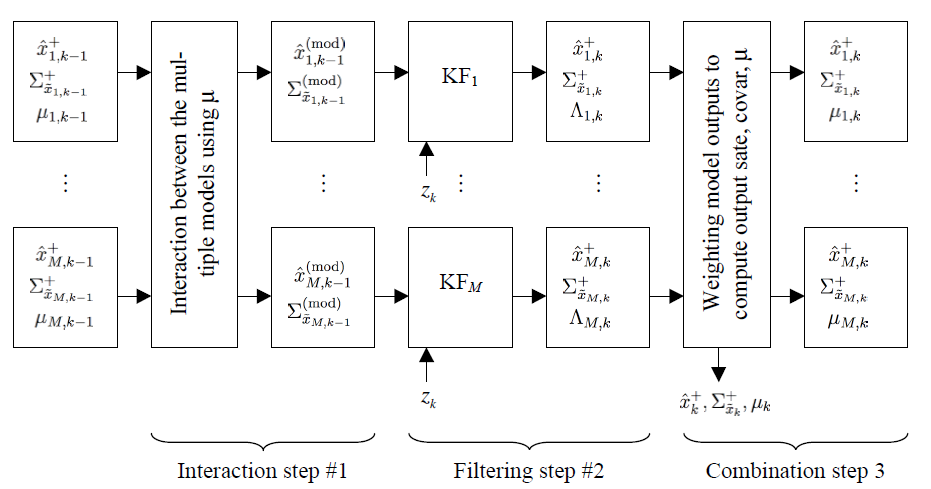
Once the basics of the Kalman filter are understood the IMM-KF is a few small steps from implementing away. A lot of the mathematic rigor is skiped here but you can look at the code in the next log to see how it works or ask me in the comments. The IMM-KF takes three high-level steps per iteration:
Step 1: interaction between the filters
The estimates and covariances from the 2 independent KFs (from the prior time step) are blended together to produce the inputs to the 2 independent KFs for the current time step. First, compute the conditional probability. Then blend together all state outputs from the prior step according to the probability that they could have contributed to the state at this time step.
Step 2: the individual filter update
After the interaction step, one time step for each of the 2 Kalman filters is executed. Both filters output the present state and covariance estimate for that mode, as well as the tendency of the present measurement given that the environment state is in the NCV mode.
Step 3: combination of filter information, yielding the output information.
Lastly, combine the results of the NCP and NCV Kalman filters for an overall environment state estimate and a probability distribution on the mode random variable. First compute the probability of being in NVC mode at time k. Next, calculate the filter output as a mixture of the individual filter estimates, according to the tendency of the environment being in the mode of that filter. Then, the state is computed as a weighted combination of the individual filter state estimates.
Here is a diagram of what this looks like (again credit for this image goes to Dr. Greg Plett from his notes at UCCS):
So, this is the algorithm we're implementing on board the STM32F4 to measure the enviroment of a particular fauna. These states along with the measurements and the measurement estimates are sent to a cloud server for further processing. This enables a high level of resolution in environments where multiple SunLeaf modules are used and very good resolution in environments where only SunLeaf one module is being used. Furthermore, this is typically a very fast algorithm for estimation and can also be implemented in higher bandwidth systems such as autonomous vehicle control systems and fun stuff like that.
-
Embedded Sensor Fusion: Part 1 The models
06/20/2016 at 18:20 • 1 commentIntroduction
I wanted to talk a little about how we are going to do manage and estimate the sensor measurements on board the STM32F4 uC. The goal of this algorithm will not only be to give an accurate measurement of the current state of the flora but it should enable us to understand the health of the flora and the environment within a certain probability. A lot of mathematics are involved in this algorithm. I'm going to be using concepts in differential equations (ODE and PDE) as well as some probability and statics. If you're just interested how we 'built' this thing you might want to move on but if you really want to see the inner workings of what we are doing to make our on-board measurements it's going to be discussed here. So, I'm going to lay it all out and if there are questions you can email me or ask them in the comments and I'll do my best to answer. First I'm going to talk a little about the model and how I derived the model. This will yield the final state space formulation. With the state space described I'll then describe the algorithm we are going to use to estimate our measurements and fuse our sensor information. Lastly, I'll put it into some Matlab simulation and we'll see how it looks when we simulate the algorithm with some real life data. (one note: I know there are not a lot of Matlab fans out there because you have to pay for it but it's what I used in college. Someday I'll port all this over to Octive but for now you're stuck with it...) I'm working on implementing the actual algorithm in the STM32F4 in C but that might take longer than this phase of the project so at least I want to talk about what we are doing and how it is a novel, scientific way to measure the health of flora.
The Model
A model in this case is a mathematical representation of how the system behaves. Many systems will have some inputs and outputs. In our case the system is the environment of the flora we are monitoring. Before the system can be modeled we need to understand a little bit about how it behaves. There are three different, measurements we are taking: light, temperature and humidity. I took some data for an environment where the flora is being kept. This data is shown below:
Light is independent of temperature and humidity. Humidity tends to depend on temperature but in a closed environment these can be treated as independent variables. Furthermore all of these variables are slow moving and a little noisy. The sensors we used to take these measurements are:
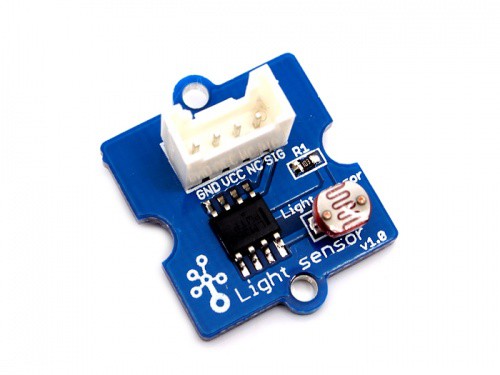
Light Sensor: Light Sensor Specs:
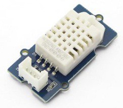
Temperature & Humidity Sensor: The famous DHT11!
These sensors all report discrete values at discrete time intervals. This means we will need to be working with discrete time models. There are a few ways to break down this system. We have the water molecules and air temperature and different aspects of light (i.e. wavelength, reflectivity, transitivity ect...) we could account for in the model. I'm concerned if I take this approach the model will become too difficult to calculate and the data won't be useful.
Instead we can observe that the temperature mostly stay in the same space and are only moved around by a few external forces such as me walking in and out of the room, it raining outside or the cat playing with the sensors. For this reason we can use a discrete "Nearly Constant Position" (NCP) model for the humidity and temperature measurements. The temperature measurement looks like there is some regular movement so if the NCP model doesn't really match the output then we'll switch to the NCV model. I may break down these measurements and look at the frequency content if there is time but for now this is what we'll use. Here's how the NCP model works:
In continuous time the model state is as follows:
Based on the data above we can then say the continuous state equations is:and the continuous output equation is:
where K is the constant temperature and humidity the room is set to. K can be calculated by taking the average of the first 10 samples.
So now let's change this to a discrete state space model. Before we do this lets clearly define the states A,B,C,D:
Since in the Z domain the C and D matrices do not change all we need to do is calculate the A and B matrices. To do this we evaluate x(t) at discrete times:and looking at the derivative of the state with the zero order hold of (k+1)T. T=300 because we are going to report every 5 minutes:Now you can do some calculus and break the integral up into two parts and you'll end up with something like this:
WhereNow the output state pretty much unchanged:
You can calculate the actual values with an inverse Laplace transform...or use Matlab:
[Ad,Bd]=c2d(A,B,T)
Now the actual values for the states are as follows.
The light measurements show a little bit different system. This system is moving at a somewhat regular rate with lots of disturbances. This looks something that can be modeled with a discrete "Nearly Constant Velocity" (NCV) model. Here's how this model works. The setup is the same as above except we are measuring the position and the velocity at which the light changes:
Everything is the same but there are no constants with the light model as the swing is between the max value, 0 and the min value 100. So the discrete state space is as follows:I omitted the D Matrix in this case because there is nothing forcing the output to a certain value. These are also the preliminary values. When I do the simulations I'll tweek them and pull some more data from our server to see if they are robust for different indoor environments.Now that we have are state spaces we can have a lot of fun. We can check for things like controllability and observability. So we have two different models: the NCP for temperature and humidity and the NCV for light. We'll need to make two different measurement estimates for these models and have these interact. We can generate different types of estimation systems and that is just what we will do in the next post.
-
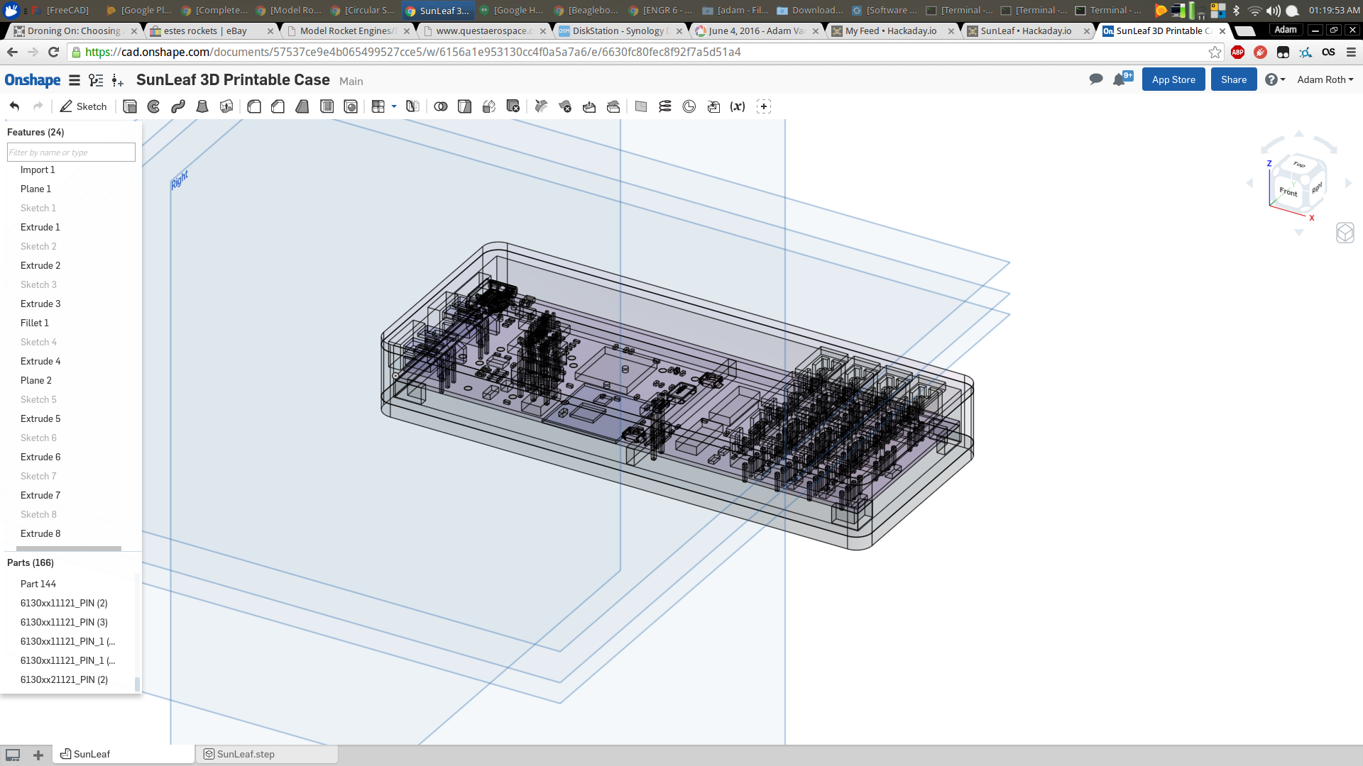
Case/Housing For SunLeaf
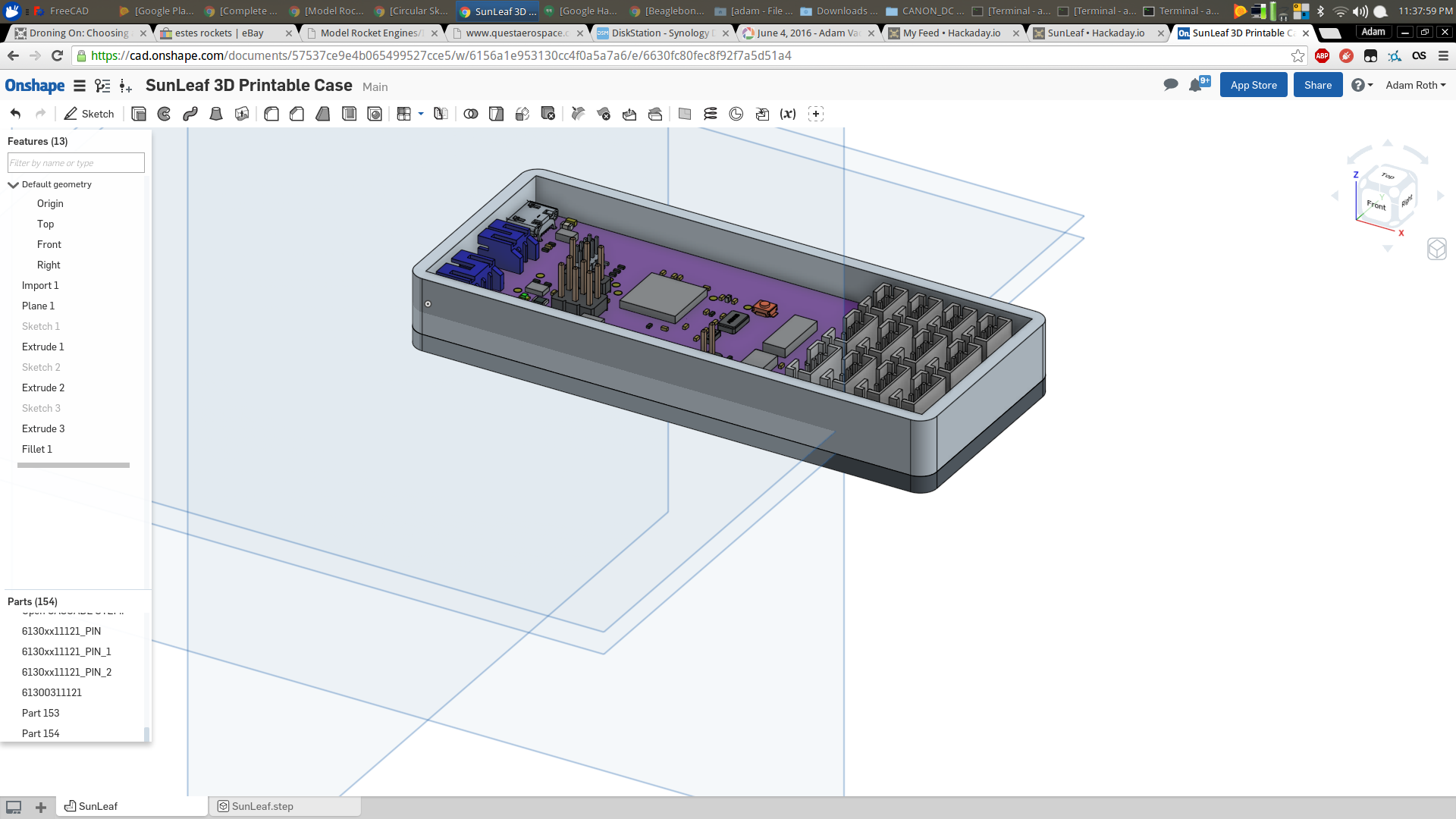
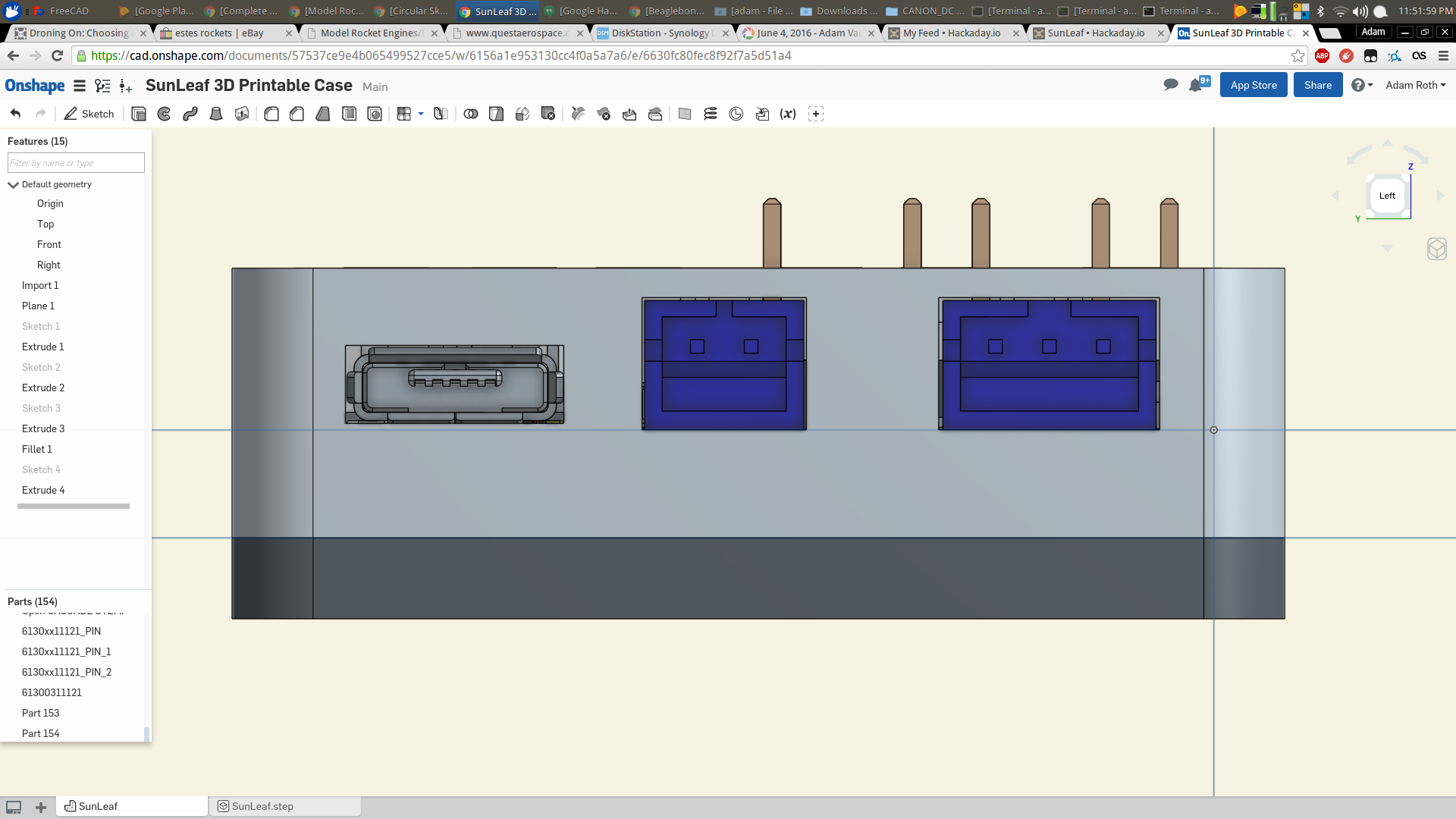
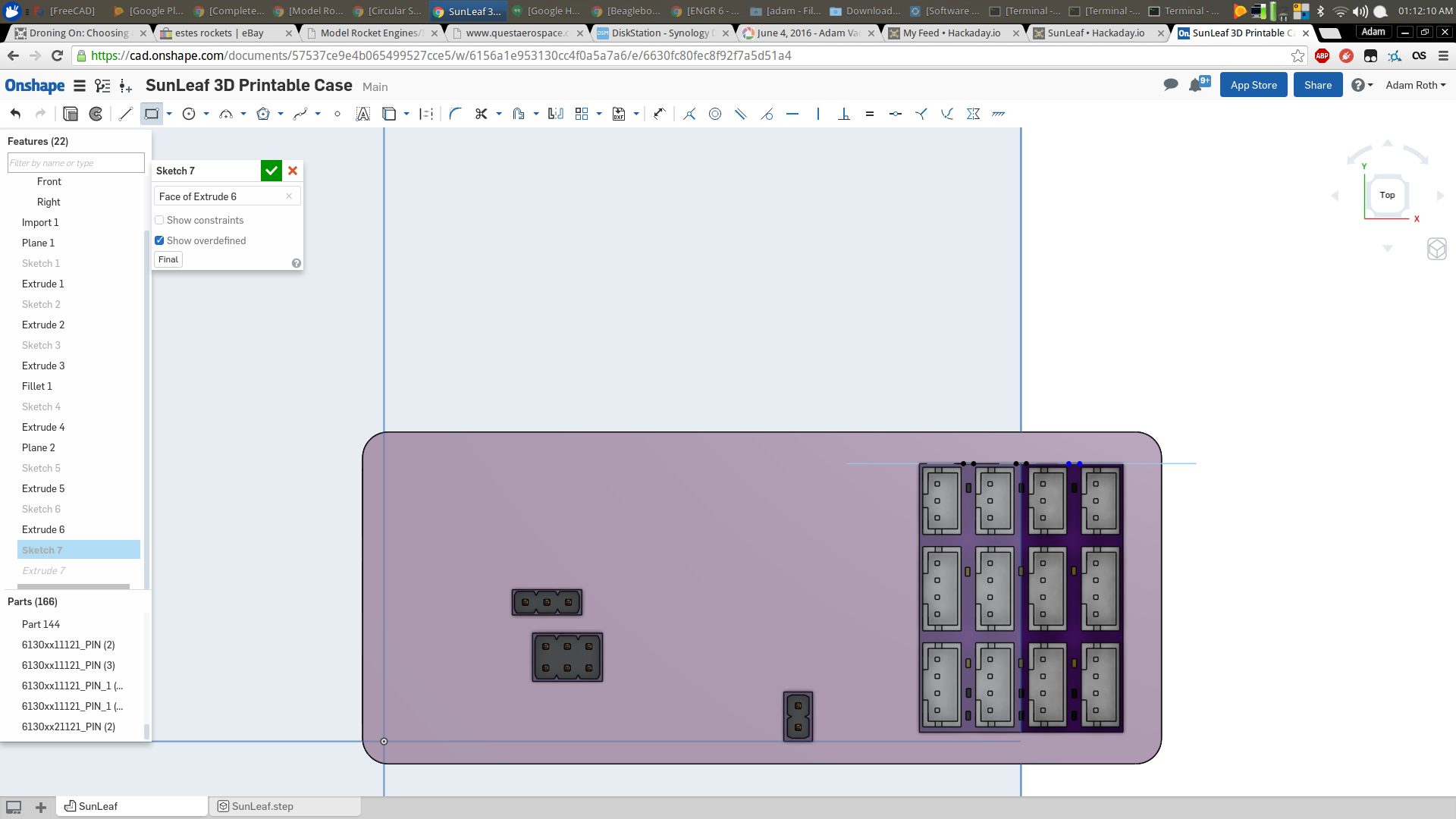
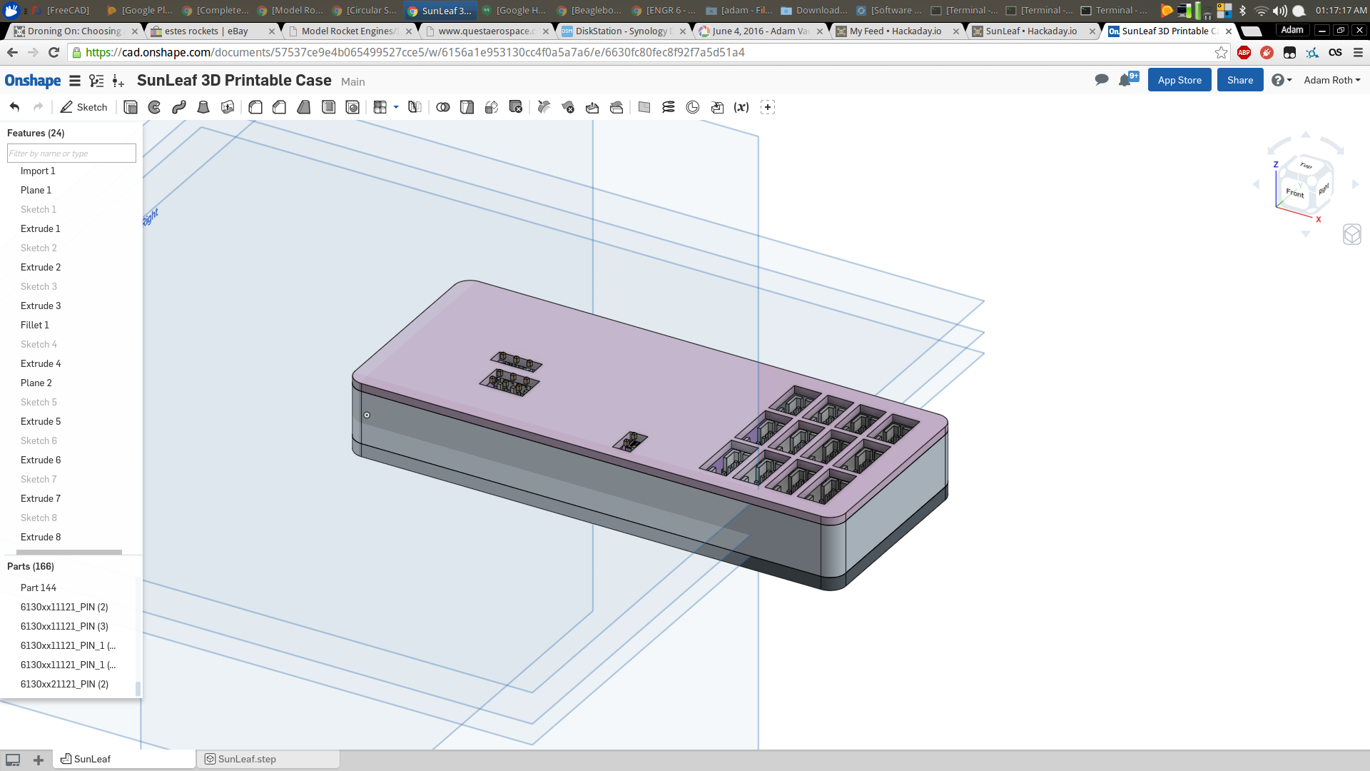
06/12/2016 at 07:01 • 0 commentsSo while we wait for the last few things to assemble the prototype SunLeaf modules I've been working on 3D printable case concepts. The goal is to develop two cases, an outdoor case with ruggedization/weather proofing and an indoor case. So far I've just been modeling a simple concept, just a lid and and bottom. The bottom mount sthe SunLeaf module with access to the back ports through cuts on the case back. The top fits into the bottom with friction fit tabs and has cutouts for all the sensor ports. Right now its just a simple housing but will evolve over time. Here is what the initial concept is looking like right now:
Back cutouts for solar panel, battery, and USB ports:
Lid :
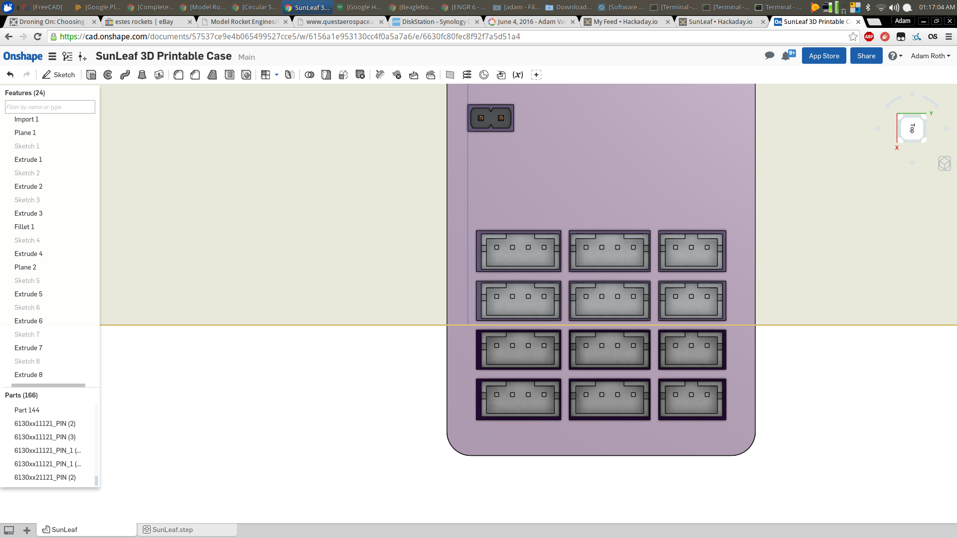
Look at the whole case:
How the SunLeaf sits within the case - translucent view
So far that's what the case is looking like. The next thing is going to be adding antenna mounting for the ESP8266 module, at the time I started working on the case CAD I didn't have the antenna's in from the mail to measure them, so in the coming days I'll be adding an antenna mount. As for an outdoor case for SunLeaf its going to be radically different, I want to mount the solar panel and battery internally and have the entire thing well sealed. This may sound crazy or ambitious but I also plan to 3D print the weather proof case as well as the indoor one. I think it can be done if we get creative with material choices and clever design. Stay tuned, there is much much more to come for SunLeaf in the coming days: assembly! Testing! and More!!
-
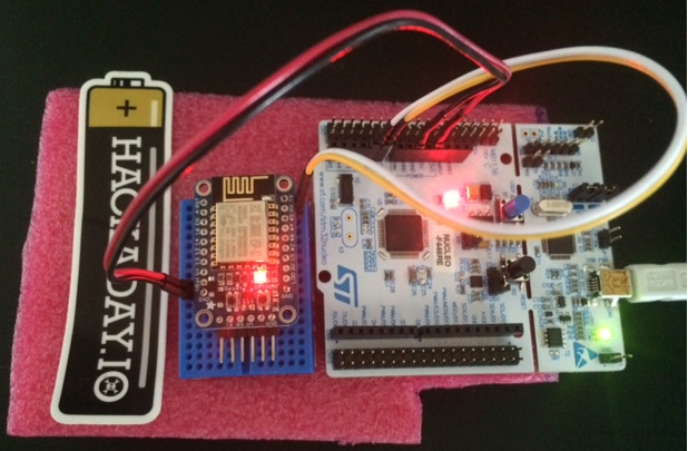
Elementary ESP to STM32 Communication
05/31/2016 at 21:10 • 3 commentsThis log is about the basic UART communication between the ESP and the STM32. For the ESP I found an awesome open-source library from Jee Labs: https://github.com/jeelabs/esp-link. I've modified the source and I'll need to do make a branch to program the STM32 Chip eventually. But this post just covers the basics: Talking between boards or basic UART functionality to make sure both tool chains are working and both boards are working the way they should. The boards are shown below. You'll notice the UART is missing from the ESP board and it is now directly connected to the STM32 dev board. According to the datasheet: https://developer.mbed.org/platforms/ST-Nucleo-F446RE/ We can use Serial 4 to communicate easily to the ESP chip. Any of the other serial ports would work but I liked the fact that the pins were next to each other. This would reduce the risk of connecting the board wrong. The white Rx on the STM32 board connects to Tx output on the ESP and the yellow TX on the STM32 board connects to the RX input. The red and black wires are power and ground, respectively.
ESP-Link
When you install the esp-link it is important to keep in mind the paths. I installed it in the /examples directory:
shane@shane-VirtualBox:/opt/esp-open-sdk/examples/esp-link$but you'll still need to edit the make files to make sure they reflect the correct build path. This is around line 70. Here is the path that worked from me.XTENSA_TOOLS_ROOT ?= /opt/esp-open-sdk/xtensa-lx106-elf/bin/I also had to edit the ESP Tool build path around line 82 to the following:ESPTOOL ?= /opt/esp-open-sdk/esptool/esptool.pyNow that the make file is ready just go ahead and type 'make'. The output is as follows if it compiles correctly.
shane@shane-VirtualBox:/opt/esp-open-sdk/examples/esp-link$ make
Makefile:73: Using SDK from /opt/esp-open-sdk/esp_iot_sdk_v1.5.2
VERSION: esp-link master - 2016-05-31 19:57:37 - development
CC mqtt/mqtt.c
CC mqtt/mqtt_cmd.c
CC mqtt/mqtt_msg.c
CC mqtt/pktbuf.c
CC rest/rest.c
CC syslog/syslog.c
CC espfs/espfs.c
CC httpd/auth.c
CC httpd/base64.c
CC httpd/httpd.c
CC httpd/httpdespfs.c
CC user/user_main.c
CC serial/console.c
CC serial/crc16.c
CC serial/serbridge.c
CC serial/serled.c
CC serial/slip.c
CC serial/uart.c
CC cmd/cmd.c
CC cmd/handlers.c
CC esp-link/cgi.c
CC esp-link/cgiflash.c
CC esp-link/cgimqtt.c
CC esp-link/cgioptiboot.c
CC esp-link/cgipins.c
CC esp-link/cgiservices.c
CC esp-link/cgitcp.c
CC esp-link/cgiwifi.c
CC esp-link/config.c
CC esp-link/log.c
CC esp-link/main.c
CC esp-link/mqtt_client.c
CC esp-link/status.c
CC esp-link/task.c
make[1]: Entering directory `/opt/esp-open-sdk/examples/esp-link/espfs/mkespfsimage'
cc -I.. -std=gnu99 -DESPFS_GZIP   -c -o main.o main.c
cc -o mkespfsimage main.o -lz
make[1]: Leaving directory `/opt/esp-open-sdk/examples/esp-link/espfs/mkespfsimage'
Compression assets with htmlcompressor. This may take a while...
Compression assets with yui-compressor. This may take a while...
ui.js            ( 37%, gzip, 2804 bytes)
pure.css         ( 22%, gzip, 3820 bytes)
console.html     ( 35%, gzip, 1188 bytes)
style.css        ( 31%, gzip, 2276 bytes)
console.js       ( 46%, gzip,  956 bytes)
services.js      ( 42%, gzip,  768 bytes)
favicon.ico      ( 29%, gzip, 71360 bytes)
log.html         ( 39%, gzip,  908 bytes)
mqtt.js          ( 41%, gzip,  736 bytes)
wifi/wifiSta.html ( 35%, gzip, 1148 bytes)
wifi/wifiAp.js   ( 41%, gzip,  948 bytes)
wifi/wifiSta.js  ( 36%, gzip, 1664 bytes)
wifi/wifiAp.html ( 31%, gzip, 1152 bytes)
wifi/icons.png   (100%, none,  428 bytes)
services.html    ( 34%, gzip, 1164 bytes)
home.html        ( 37%, gzip, 1972 bytes)
mqtt.html        ( 36%, gzip, 1200 bytes)
96 -rw-rw-r-- 1 shane shane 95012 May 31 19:57 build/espfs.img
AR build/httpd_app.a
LD build/httpd.user1.out
Dump : /opt/esp-open-sdk/xtensa-lx106-elf/bin/xtensa-lx106-elf-objdump -x build/httpd.user1.out
Disass: /opt/esp-open-sdk/xtensa-lx106-elf/bin/xtensa-lx106-elf-objdump -d -l -x build/httpd.user1.out
FW firmware
ls -ls eagle*bin
  4 -rwxrwxr-x 1 shane shane   3013 May 31 19:57 eagle.app.v6.data.bin
320 -rwxrwxr-x 1 shane shane 326584 May 31 19:57 eagle.app.v6.irom0text.bin
 16 -rwxrwxr-x 1 shane shane  13496 May 31 19:57 eagle.app.v6.rodata.bin
 32 -rwxrwxr-x 1 shane shane  31728 May 31 19:57 eagle.app.v6.text.bin
-1333811629
1333811628
** user1.bin uses 374900 bytes of 503808 available
LD build/httpd.user2.out
-1071342667
1071342666
shane@shane-VirtualBox:/opt/esp-open-sdk/examples/esp-link$
Next put your serial connected ESP into programming mode and flash it using esptool:esptool.py --port /dev/ttyUSB0 --baud 460800 write_flash -fs 32m -ff 80m \ 0x00000 boot_v1.4\(b1\).bin 0x1000 user1.bin 0x3FE000 blank.binA few notes on this command. If you are having trouble getting esptool to connect to the ESP8266 then try slowing down the baud speed. 460800 baud seems to work ok on little examples like 'blinky' but for bigger examples issues occur connecting and syncing. Also, it is important to make sure you are flashing the correct part of your memory. See this link for details:
http://www.espressif.com/en/support/explore/get-started/esp8266/getting-started-guide#
That was the hard part.
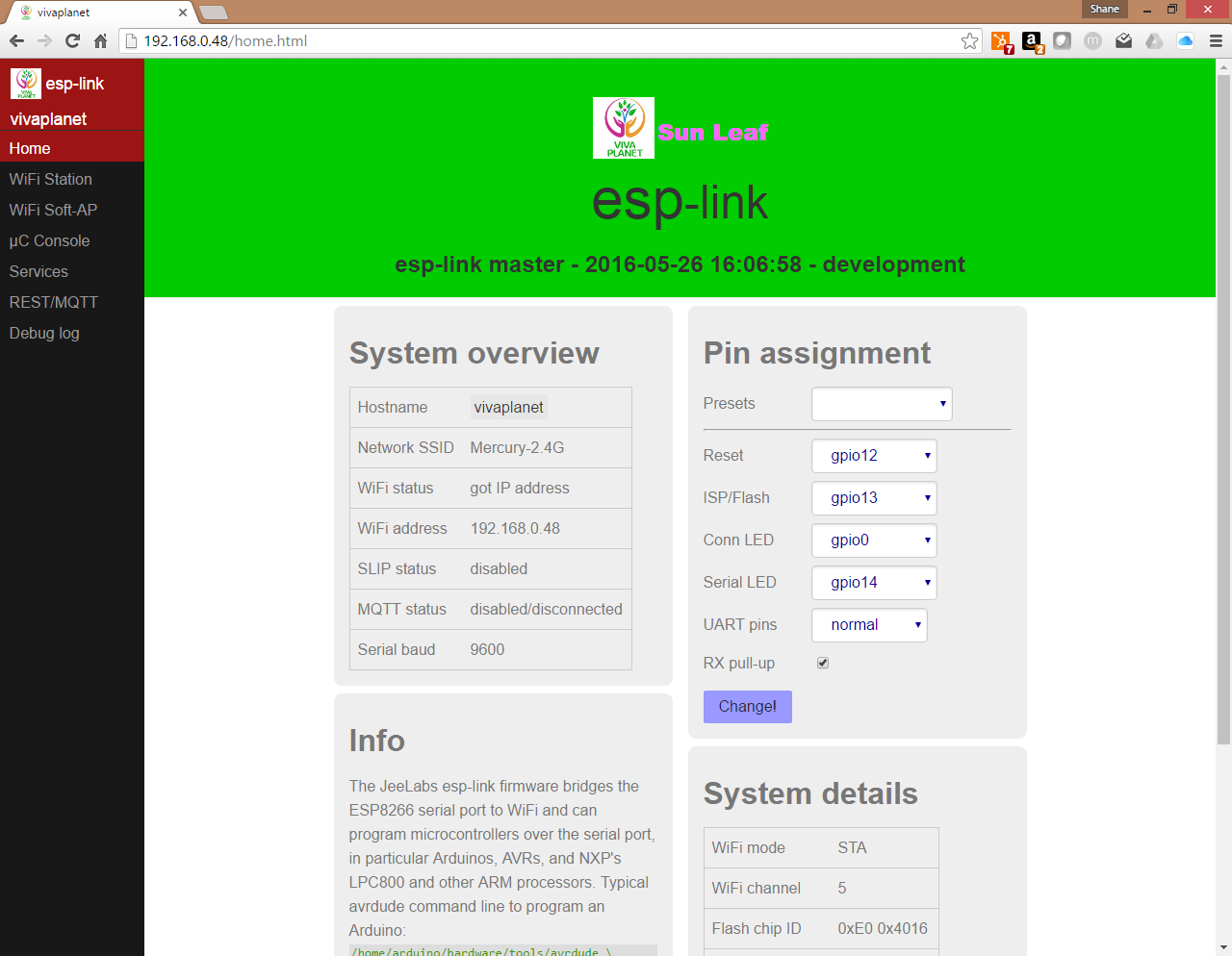
Next go here: https://github.com/jeelabs/esp-link#wifi-configuration-overview and configure the ESP. By now I hope you've realized that this is a really nice package to start with.
After you go through and configure the wifi correctly you can do OTA updates and iterate changes quickly. Below shows the ESP splash page for SunLeaf. I changedsome of the colors that Jee Labs uses because even though their code is awesome I didn't really like their color scheme.
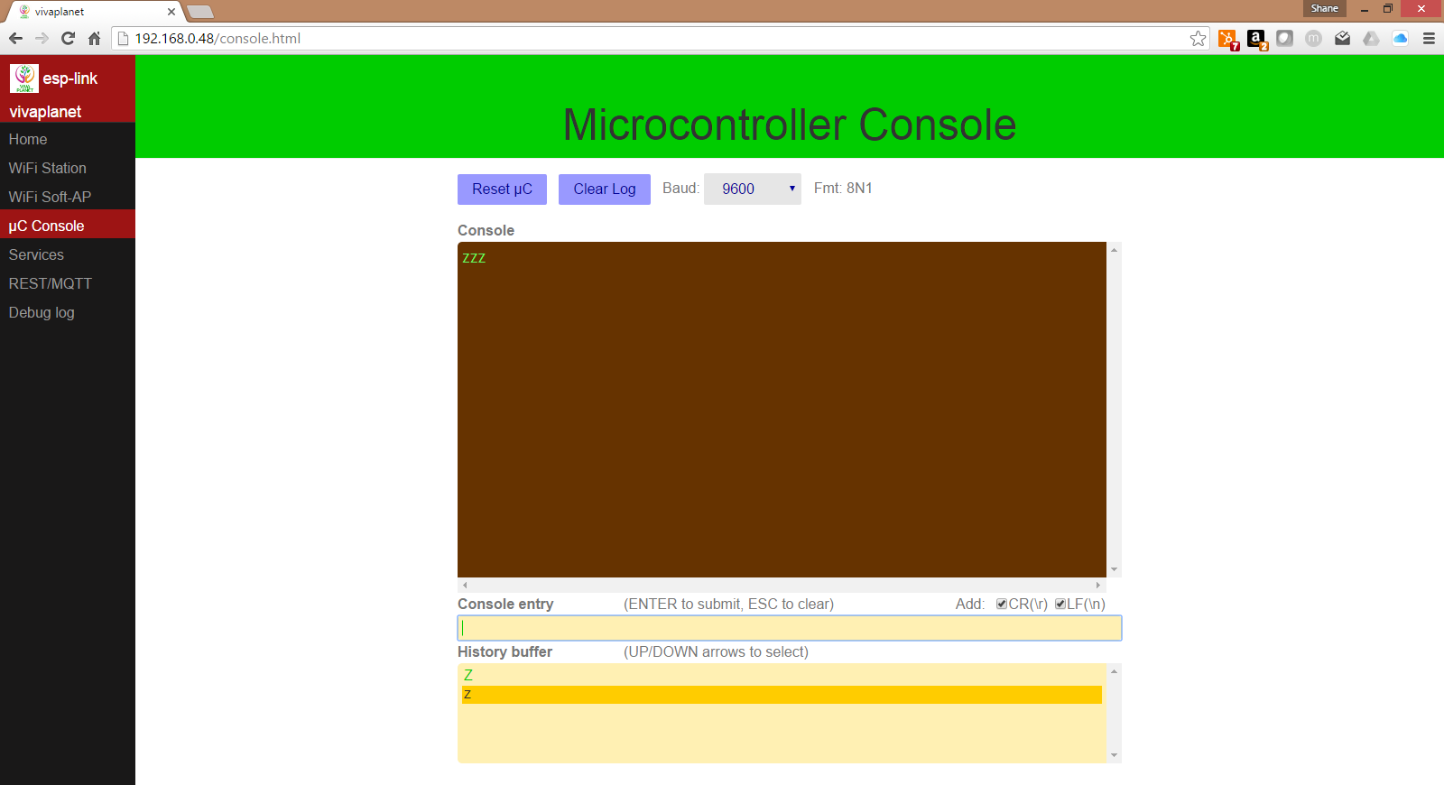
Aslo notice the menu bar on the side has a 'uC Console' page. This is the page we will use to talk to the STM32. So now tht you've set up the ESP it's time to dive into to the STM32 Nucleo board.
STM32 mBed.org
I am using the Nucelo-F446RE Development board. You can just get the drivers and plug the thing into your pc. It should recognize the file. When you open the file in good browser it will take you to the mbed.org site. This site has an online IDE that will allow you to flash the STM32. It is really nice as well.
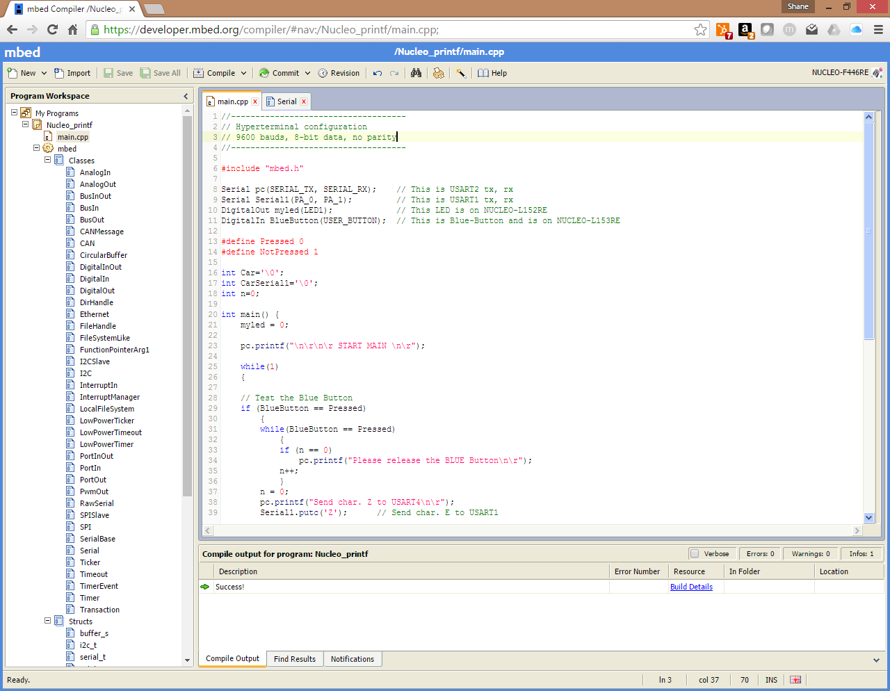
There is a built in UART example that I started with on mBed.org. I wanted to send a character to the ESP and have the character display on my PC. I found a version of the code here: http://www.emcu.it/NUCLEOevaBoards/U2andU1onL152/U2andU1onL152.html and I modified it to use on my board.
For completeness here is the actual code:
//------------------------------------
// Hyperterminal configuration
// 9600 bauds, 8-bit data, no parity
// for the F446RE only
//------------------------------------

#include "mbed.h"

Serial pc(SERIAL_TX, SERIAL_RX);    // This is USART2 tx, rx
Serial Serial1(PA_0, PA_1);         // This is USART1 tx, rx
DigitalOut myled(LED1);             // This LED is on NUCLEO-L152RE
DigitalIn BlueButton(USER_BUTTON);  // This is Blue-Button and is on NUCLEO-L153RE

#define Pressed 0
#define NotPressed 1

int Car='\0';
int CarSerial1='\0';
int n=0;

int main() {
    myled = 0;

    pc.printf("\n\r\n\r START MAIN \n\r");

    while(1)
    {

    // Test the Blue Button
    if (BlueButton == Pressed)
        {
        while(BlueButton == Pressed)
            {
            if (n == 0)
                pc.printf("Please release the BLUE Button\n\r");
            n++;
            }
        n = 0;
        pc.printf("Send char. Z to USART4\n\r");
        Serial1.putc('Z');      // Send char. E to USART1
        }

    // Test the char. received from USART2 tha is USB Virtual COM
    if(pc.readable())
        {
        Car = pc.getc();
        if (Car == 'Z')
            {
            pc.printf("Send char. Z (received from USB_VirtualCOM) to USART4\n\r");
            Serial1.putc('Z');  // Send char. E to USART1
            }
        Car = '\0';
        }

    // Test the char. received from USART1
    if (Serial1.readable())
        {
        CarSerial1 = Serial1.getc();    // Get char. from USART1
        if (CarSerial1 == 'Z')
            {
            pc.printf("RX char. Z from USART4\n\r");
            myled = 1;
            wait(1);
            }
        myled = 0;
        CarSerial1 = '\0';
        }

    }
}
Now you can just press compile. The code will upload to the STM32 and you'll be able to see it in the ESP Micro-controller console.
Putting it all together
You should have your ESP and STM32 wired as shown at the top of this page. If it is and you've used the code shown above you can send the Z character back and forth! I know you've always dreamed of sending Z's over wifi and now you can...
Here is what it looks like on the ESP Micro-controller console.
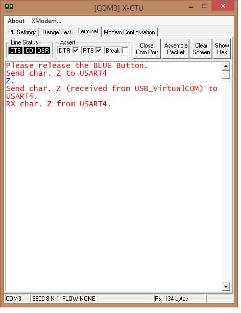
Here is what it looks like on the PC from a terminal (I used X-CTU but really anything like putty, teraterm or hyperterminal would work).The next embedded systems post is going to be a little more complicated. We are going to (attempt) to address programming the STM32 with the ESP-Link. They don't currently have this functionality but why not add it? :-)
-
Quick Update: BOM & Components Ordered
05/25/2016 at 23:07 • 2 commentsSo today the BOM (bill of materials for the uninitiated) is posted. This is only the prototype BOM, so some components are left out, later those components will be published once building and testing is complete. The BOM is below:
SunLeaf BOM
Designator Value Package Quantity Digikey # MFR # Price Comment C31 0.01uF C0603 1 490-8269-1-ND GRM1857U1A103JA44D Murata Electronics North America 0.03580 @ 4000 CAP CER 10000PF 10V U2J 0603 C4, C7, C10, C11, C12, C13, C14, C18, C19, C20, C21, C22, C23, C24, C25, C26, C27, C28, C29, C30, C33 0.1uF C0402 21 1276-1506-1-ND CL05B104JP5NNNC Samsung Electro-Mechanics America, Inc. 0.00758 @ 10,000 CAP CER 0.1UF 10V X7R 0402 R1 1M R0402 1 1276-3433-1-ND RC1005F105CS Samsung Electro-Mechanics America, Inc. 0.00137 @ 10000 RES SMD 1M OHM 1% 1/16W 0402 R2, R3, R4, R5, R19, R20, R21, R22, R33 1k R0402 9 1276-3430-1-ND RC1005F102CS Samsung Electro-Mechanics America, Inc. 0.00137 @ 10,000 RES SMD 1K OHM 1% 1/16W 0402 C15, C16 1uF C0402 2 1276-1445-1-ND CL05A105KA5NQNC Samsung-Electro-Mechanics-America,-Inc. 0.04830 @ 10000 1µF ±10% 25V X5R Ceramic Capacitor -55°C ~ 85°C Surface Mount, MLCC 0402 (1005 Metric) 0.039" L x 0.020" W (1.00mm x 0.50mm) R7, R8 2k R0805 2 1276-5287-1-ND RC2012F202CS Samsung-Electro-Mechanics-America,-Inc. 0.00266 @ 5000 RES SMD 2K OHM 1% 1/8W 0805 C32 4.7uF C0402 1 1276-1481-1-ND CL05A475KQ5NRNC Samsung Electro-Mechanics America 0.08 @ 10000 CAP CER 4.7UF 6.3V X5R 0402 R11, R12, R13, R14, R15, R16, R17, R18, R27, R28 4k7 R0402 10 1276-3466-1-ND RC1005F472CS Samsung Electro-Mechanics America, Inc. 0.00137 4.7k Ohm ±1% 0.063W, 1/16W Surface Mount Resistor Thick Film ±100ppm/°C 0402 (1005 Metric) X2 8MHZ ABM3B8.000MHZB2T 1 535-9720-1-ND ABM3B8.000MHZB2T Abracon LLC 0.30450 @ 5000 8MHz ±20ppm Crystal 18pF 200 Ohm 20° C ~ 70°C Surface Mount 4SMD, No Lead (DFN, LCC) C5, C6 9pF C0402 2 1276-1616-1-ND CL05C090CB5NNNC Samsung Electro-Mechanics America, Inc. 0.00462 @ 10,000 CAP CER 9PF 50V NP0 0402 R6, R26 10K R0402 2 1276-3431-1-ND RC1005F103CS Samsung Electro-Mechanics America, Inc. 0.00137 @ 10000 RES SMD 10K OHM 1% 1/16W 0402 C2, C3 18pF C0402 2 1276-1647-1-ND CL05C180GB5NCNC Samsung Electro-Mechanics America, Inc. 0.00756 @ 10,000 CAP CER 18PF 50V NP0 0402 R23, R24 22r R0402 2 A102720TR-ND CPF0402B22RE1 TE Connectivity AMP Connectors 0.10921 @ 1000 RES SMD 22 OHM 0.1% 1/16W 0402 R25 47K R0402 1 1276-4416-1-ND RC1005J473CS Samsung Electro-Mechanics America, Inc. 0.00137 @ 10000 RES SMD 47K OHM 1% 1/16W 0402 C1 47pF C0402 1 1276-1697-1-ND CL05C470FB5NNNC Samsung-Electro-Mechanics-America,-Inc. 0.01335 @ 5000 47pF ±1% 50V C0G, NP0 Ceramic Capacitor -55°C ~ 125°C Surface Mount, MLCC 0402 (1005 Metric) 0.039" L x 0.020" W (1.00mm x 0.50mm) U5 74HC4052 1 568-1456-1-ND 74HC4052D,653 NXP-Semiconductors 0.13695 @ 2500 IC MUX/DEMUX DUAL 4X1 16SOIC R9 100K R0402 1 Standin O603 N/A Standin 0402 R29, R30, R31, R32 200 ohm R0402 4 1276-3959-1-ND RC1005F201CS Samsung Electro-Mechanics America, Inc. 0.00203 @ 10K RES SMD 200 OHM 1% 1/16W 0402 RN1, RN2, RN3, RN4 200 ohm EXB-N8V201JX - CAC-50P200X100-8N 4 Y10201CT-ND EXB-N8V201JX Panasonic Electronic Components 0.00842 @10000 RES ARRAY 4 RES 200 OHM 0804 C17 10uF C0603 1 1276-1038-1-ND CL10A106KQ8NNNC Samsung Electro-Mechanics America, Inc. $0.05145 CAP CER 10UF 6.3V X5R 0603 J2 FTSH-105-XX-X-DV 1 609-3695-1-ND 20021121-00010C4LF Amphenol FCI 0.32 @ 15000 20021121-00010C4LF ARM COrtex JTAG P2 61300211121 61300211121 1 732-5315-ND 61300211121 Wurth-Electronics-Inc 0.08910 @ 500 2 Positions Header, Unshrouded Connector 0.100" (2.54mm) Through Hole Gold P3 61300311121 61300311121 1 732-5316-ND 61300311121 Wurth-Electronics-Inc 0.10396 @ 500 3 Positions Header, Unshrouded Connector 0.100" (2.54mm) Through Hole Gold P1 61300621121 61300621121 1 732-5295-ND 61300621121 Wurth-Electronics-Inc 0.38610 @ 500 6 Positions Header, Unshrouded Connector 0.100" (2.54mm) Through Hole Gold X1 ABS07-32.768KHZ-9-T ABS07-32.768KHZ-9-T 1 535-9544-1-ND ABS07-32.768KHZ-9-T Abracon LLC 0.18000 @ 3K 32.768kHz ±20ppm Crystal 9pF 70 kOhm -40°C ~ 85°C Surface Mount 2-SMD J13, J14, J15, J16 B3B-PH-K-S(LF)(SN) B3B-PH-K-S(LF)(SN) 4 455-1705-ND B3B-PH-K-S(LF)(SN) JST $0.19 CONN HEADER PH TOP 3POS 2MM SW1, SW2 B3U-1000P B3U-1000P 2 SW1020CT-ND B3U-1000P OMRON 0.55 @7000 SWITCH TACTILE SPST-NO 0.05A 12V J5, J6, J7, J8, J9, J10, J11, J12 B4B-PH-K-S(LF)(SN) B4B-PH-K-S(LF)(SN) 8 455-1706-ND B4B-PH-K-S(LF)(SN) JST $0.24 CONN HEADER PH TOP 4POS 2MM D1 BAT20JFILM - DIOM1712X11N BAT20JFILM - DIOM1712X11N 1 497-3381-1-ND BAT20JFILM ST Microelectronics $0.44 DIODE SCHOTTKY 23V 1A SOD323 D4, D5 BAV70S BAV70S 2 568-5004-1-ND BAV70S,115 NXP 0.055 @ 15K DIODE ARRAY GP 100V 250MA 6TSSOP FB1 BLM15HG601SN1D BLM15HG601SN1D 1 490-3998-1-ND BLM15HG601SN1D Murata Electronics North America 0.05090 @ 10000 FERRITE BEAD 600 OHM 0402 1LN U2 bq24210 - QFN50P300X200X80-10N bq24210 - QFN50P300X200X80-10N 1 296-28738-1-ND BQ24210DQCT Texas Instruments 1.46250 @ 1250 IC BATT CHARGER LI-ION 10WSON (USB & SOLAR Input) Q1 DMG2307L-7 - SOT92P240X102-3N DMG2307L-7 - SOT92P240X102-3N 1 DMG2307L-7DICT-ND DMG2307L-7 Diodes-Incorporated 0.08100 @ 3000 MOSFET P-CH 30V 2.5A SOT-23 J1 DX4R005J91R5100 DX4R005J91R5100 1 WM17143CT-ND 475890001 0.50808 @ 500 Micro USB Jack B DA11 ESDA6V1BC6 ESDA6V1BC6 1 497-6635-1-ND ESDA6V1BC6 STMicroelectronic 0.126 @ 15K TVS DIODE 5VWM SOT23-6 IC1 ESP8266 ESP-02 ESP8266 ESP-02 1 Ebay includes antenna ESP-02 ESP8266 ESP-02 WIFi SoC Module D2 LED Green LED0603_GREEN 1 160-1446-1-ND LTST-C191KGKT Lite-On Inc. 0.03760 @ 5000 LED GREEN CLEAR 0603 SMD D3 LED Orange LED0603_ORANGE 1 160-1445-1-ND LTST-C191KFKT Lite-On Inc. 0.03760 @ 5000 LED ORANGE CLEAR 0603 SMD FB2 MI0603K300R-10 MI0603K300R-10 1 240-2373-1-ND MI0603K300R-10 Laird-Signal Integrity Products 0.01920 @ 4000 FERRITE BEAD 30 OHM 0603 1LN U4 PCA9518DBQR PCA9518DBQR 1 296-22764-1-ND PCA9518DBQR Texas Instruments 0.95062 @ 1000 IC EXPANDABLE 5CH I2C HUB 20QSOP DA1, DA2, DA3, DA4, DA5, DA6, DA7, DA8, DA9, DA10 SOT95P230X110-3N SOT95P230X110-3N 10 568-4041-1-ND PESD3V3L2BT,215 NXP Semiconductors 0.14067 @ 15,000 TVS DIODE 3.3VWM 26VC SOT23 R10 487 R0402 1 1276-3991-1-ND RC1005F4870CS Samsung Electro-Mechanics America, Inc. 0.00203 @ 10K RES SMD 487 OHM 1% 1/16W 0402 J3 S2B-PH-K-S(LF)(SN) S2B-PH-K-S(LF)(SN) 1 455-1719-ND S2B-PH-K-S(LF)(SN) JST $0.17 CONN HEADER PH SIDE 2POS 2MM J4 S3B-PH-K-S(LF)(SN) S3B-PH-K-S(LF)(SN) 1 455-1720-ND S3B-PH-K-S(LF)(SN) JST $0.17 CONN HEADER PH SIDE 2POS 2MM U1 STM32F446RET6 - TSQFP50P1200X1200X160-64N STM32F446RET6 - TSQFP50P1200X1200X160-64N 1 497-15376-ND STM32F446RET6 ST Microelectronics U3 TLV1117LV - SOT230P700X180-4N TLV1117LV - SOT230P700X180-4N 1 296-28778-1-ND TLV1117LV33DCYR Texs Instruments 0.27 @ 1000 IC REG LDO 3.3V 1A SOT223 TP1, TP2 Alligator-TP Alligator-TP 2 Adam Vadala-Roth Socket TP3, TP4, TP5, TP6, TP7, TP8, TP9, TP10, TP11, TP12, TP13, TP14 TP-2 TP-2 12 Socket Also I have gotten notice from @oshpark that the panel the SunLeaf boards were on got sent to the fab yesterday, PCBs will be in the mail in about 10 days, I estimate a similar arrival for the components from digikey. When all arrives I will be hand assembling the first three SunLeaf modules under a microscope. Last thing, the BOM is available in open document format in the files section of the project page. Stay tuned for more soon!
-
SunLeaf is Off to Fab @ OSHPark!
05/20/2016 at 01:11 • 0 commentsSo today the first SunLeaf prototypes were ordered from @oshpark using their 4 layer prototyping service. PCBs should take about two weeks, in the mean time I will be ordering components from Digikey and setting up the SMT soldering tools I acquired over the winter.
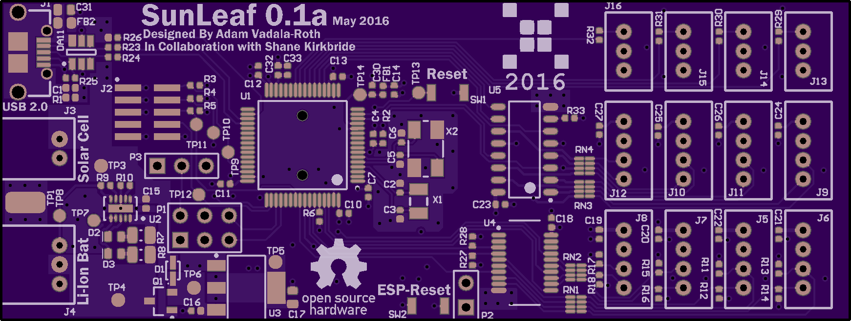
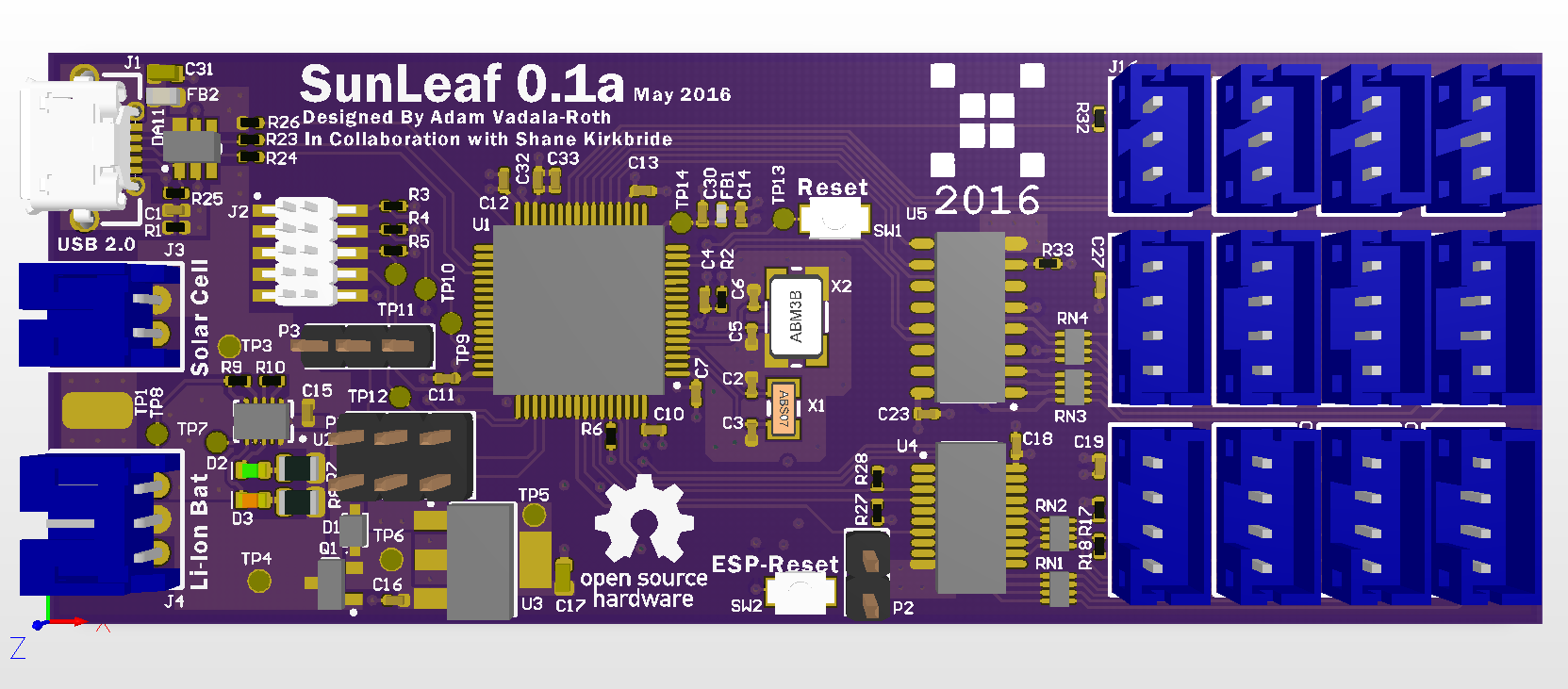
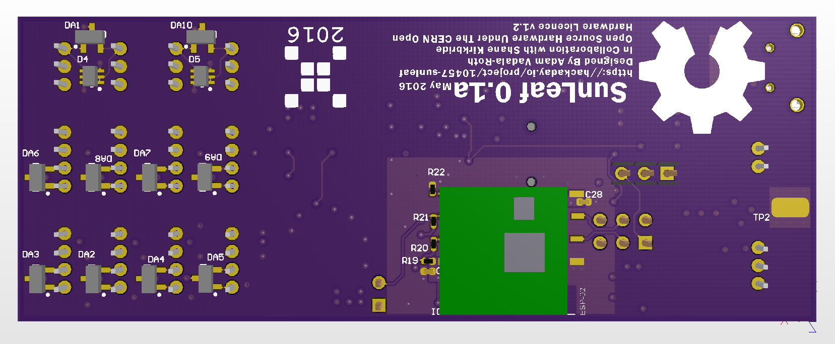
PCB Renders From OSHPark:Top
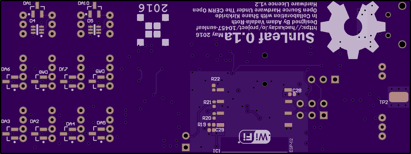
Bottom
3D Render in OSHPark Purple
Top
Bottom
Stay tuned for future updates on the BOM, and assembly!
SunLeaf
A solar powered wireless picopower sensor module with cloud Datalogging and control geared towards agriculture and environmental monitoring