QuickSilver Neo: Open Source GPU

Ordinary textures were just a bit to big to really work effectively. Anything we can do to make make them smaller in memory would be a great boon. We're already working at 8 bits per pixel precision though, so we can't really reduce that any further if we want to stay above EGA quality. Instead, we'll apply compression to the textures.

You may be familiar with image compression as used on the web or the desktop, typically in either JPEG or PNG format. These are great at reducing the size of an image by factor of 10 to 100 or more, while still keeping great image quality. Unfortunately, these algorithms are not a great fit for texture compression. Texture compression needs two important properties:

• Quick and simple to decode. We need to do this on-the-fly, in hardware, so we don't have the time or space to do a full decoding of JPEG or PNG.
• Random access. Triangles can start rendering anywhere, and we don't know in advance which part will be used, so we should have access to each individual texel without too much overhead. JPEG and PNG pretty much require the decoding of the entire image at once.
  

Those two are very important to get right. On the other hand, we don't really care about the following:

• Compression rate. Better compression is nice of course, but we'll take any gains we can. Even a factor of two would be great.
  
• Encoding speed. Textures are typically compressed just once: when they are created. This is done offline and way before we use them, so we can take as long as we need.
  

To make random access times lower, texture compression is usually done in blocks of a few pixels, with each block always the same size so you know exactly where to find it. We'll use the most common size: 4x4 texels. Let's draw the block so we know where we start:

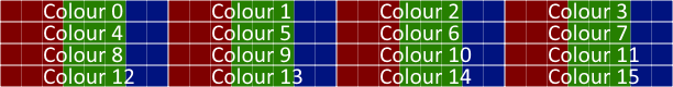
Block-based compression algorithms basically assume that pixels in an image look a lot like the pixels that surround them. S3 Texture Compression 1, also known as DXT1 in one such algorithm. Instead of storing all 16 colours it stores just 2 colours Ca and Cb per 4x4 pixel block. Then, for each pixel in the block it has an index value that chooses one of those two colours. To make gradients (which are pretty common in many types of images) look a bit better, each index can also choose between a blend of the two colours, giving 4 options: Colour a, Colour b, ⅓ Ca + ⅔ Cb, and ⅓ Cb + ⅔ Ca. This gives the following encoding (note that DXT1 uses 16 bits per colour):

Because QuickSilver outputs at just 8 bits per pixel, and because it will probably use pretty small textures where every bit of detail counts, I've chosen for a slightly different trade-off. Instead of using 2 16-bit colours and adding two intermediate values, basic QuickSilver Texture Compression uses 4 8-bit colours. This trades colour precision for colour variety, something I think would be more valuable for very small textures.

We now use 64 bits for every 16 pixels, or just 4 bits per pixel, halving our original bandwidth and storage requirements. An improvement on all fronts? Almost. While the average amount of data we need per pixel has halved, the minimum amount has increased by a factor 8, as we now need to fetch an entire block to read even a single pixel from the image. Fortunately, the properties of the on-board RAM eases the pain a little. The RAM actually uses 16-bit data words, and the time between sequential accesses is much lower than the random access penalty. A random word read requires 70 ns, but 4 sequential words can be read in 120ns, less than twice the amount.

We do get a lot more pixels for those 120 ns. In a future post I'll talk about using a cache to make use of those extra pixels.

Enough formula and bit-counting, let's get to something more exciting: Texture Mapping!

Texture mapping is, at its core, pretty straightforward. You have a image (the texture) you want project onto your triangle. The texture has horizontal and vertical coordinates U and V. For a triangle, you can take the (U,V) coordinates at each vertex, and just interpolate to get the coordinates at each point within the triangle. Then, when drawing the triangle, instead of directly drawing a colour we instead calculate the (U,V) coordinates, look up the corresponding texture element (texel), and use that colour to draw to the screen.

Pretty simple, right? We can actually already do this in QuickSilver, just use the R and G values as the U and V coordinates, put some memory nearby to place our texture, look up the texel, and output to the screen. Unfortunately, this approach is both theoretically incorrect and practically infeasible. We'll ignore the theory, and solve the practical.

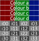
Alright, so that is a bit of a bold claim, let me explain the theoretical incorrectness and why we'll ignore it. The simple linear interpolation I talked about above great for triangles that are viewed straight on, flat relative to the screen, but it doesn't work for triangles to have some depth to them. Compare it to a brick wall. When you take a photograph of the wall straight on, each brick will be the same size on the photograph. Take a picture of the same wall from an angle, thought, and the bricks that are close will appear larger than those that are further away. A simple linear interpolation would render each brick as equally wide on the photograph. This is called "affine texture mapping". Wikipedia has a nice image comparing it to the correct version:

The trick to correct this uses an interesting property: while you can't interpolate Z, or the U,V coordinates, linearly over the screen, you can linearly interpolate 1/Z, U/Z and V/Z. Then when you want to render a pixel you just divide the values of U/Z and V/Z by 1/Z to get the correct U and V.

We're not going to do that. It's a simple fix, I know, but it requires two additional divisions (or one reciprocal and two multiplications) for every pixel. And dividers in hardware are bulky and slow. Instead, we'll follow the great example of the Sony Playstation and Sega Saturn in just completely ignoring perspective correctness and render everything with affine mapping.

The second part of the problem is more practical (with loads more little details further along the line.) Storage and bandwidth limitations once again rear their ugly little heads. Let's start by calculating how much of each we'll expect to need.

Seeing how the VGA output on the Nexys 2 board only has 8 bits per pixel, I'll use the same limit on the textures. As a minimum, I'd would like to display one unique texel per pixel. The 640x480 resolution runs at a pixel-clock of 25MHz, but the actual time between scanlines is a bit longer due to the horizontal blanking times. If you include the blanking time it comes to an equivalent of 800 pixels per scanline, so we have (800/640) / 25MHz = 50ns per texel, or 20MBytes/s.

As always, we can choose between two extremes: the very fast but small Block RAM, or the large but slow on-board RAM. The BRAM is easy to interface and can easily meet the bandwidth requirements. Even in the most optimistic situation, can only use 16 BRAM for texture storage, which at 2KByte per BRAM means a total of 32KByte of texture memory, or a total texture space of about 256x128 texels. That's small even for a single texture, but this would have to be shared among all textures on the screen.

The on-board RAM is much bigger. At 16MByte it could fit a whopping 4096x4096 texels. It's random access latency is rather high at 70ns, though. Too large to read the textures at the rate we would like, and that's before we even considered doing anything else with the RAM.

In the next post, I'll talk about how texture compression can be applied to reduce both storage and bandwidth requirements for textures. After that I'll talk about how I use caching to combine the benefits of both types of memory.

Before going any further, we have a few bits to clarify. Specifically, the bits used to represent all the values in the pipeline. First I'll talk about the sizes for each individual variable in the system. Then, I'll look at a few of the main memories I need to implement the pipeline up to this point.

As always, QuickSilver is defined by the imitations of its platform. While higher resolutions would be nice, I'll stick to 640x480 and spend more time on producing prettier pixels, rather than more pixels. Besides, the 25MHz pixel clock is a nice even division of the 100MHz base clock of QuickSilver. With a resolution of 640x480, we need at least 10 bits for the X-coordinate, and 9 for the Y-coordinate. For symmetry's sake, let's put both at 10. I wanted to look at getting some sub-pixel precision, so I added 2 more bits to each to represent 'quarter' pixels. This may or may not work out in testing, so I'm not promising anything!

The Z-coordinate is a bit trickier. The reason to store Z even after projecting all triangles to a 2D plane is to order them on screen using a Z-buffer. This means we'll need enough precision to differentiate between two objects close to each other, and consistently decide which is closer to the camera. Lack of precision results in what is called "Z-fighting", two objects that are pretty much at the same depth fighting over which gets to be on top, with the outcome varying per frame, and even per pixel. Unfortunately, lack of Z-buffer precision is just something we have to deal with, even on more modern GPUs. So in this case I'll take the "shoulders of giants" approach and just copy what early 3D accelerators did: 16-bits for Z.

(For some more background on the problems with z-accuracy, check out this article by Steve Baker: https://www.sjbaker.org/steve/omniv/love_your_z_buffer.html )

The VGA connection on the Nexys 2 board I'm using to develop QuickSilver only has a 332-RGB connection: 3 bits for red, 3 for green and 2 for blue, for a total of 8 bits. We could just accept this, but I do want a bit more precision than that. Besides, I also want to reuse these components when I'll implement texture mapping, using R and G as the U and V coordinates respectively. As a nice compromise between size and scope, I've decided on 12 bits for R and G, and 8 for B. This gives us a total 4096x4096 texture space, with 8 bits for whatever (shading maybe?). And it all sums nicely to 32.

In summary, for the input triangles:

The PreCalc produces a few more values. Specifically, the m and n gradients, and the intermediate Q value. The gradients represent changes in the components over the screen. To represent these values, we can't just use integers, we would need some fractional numbers as well. These days, most computers use floating-point notation, similar to scientific notation. In it, you separate the digits of a value and its order of magnitude into to numbers: the significand and the exponent. In decimal you could write 123.45 as 1.2345 * 10². This representation is very flexible, allowing both very small and very large numbers in a very small number of bits. Unfortunately, working with it is rather complicated and expensive in hardware.

Instead we'll use the far simpler fixed-point notation. Basically, take whatever I write down and put the decimal point in a specific place. Using the same example as before, again in decimal, I say that I'll always use 4 numbers before the decimal point, and 4 behind. 123.45 would then be written as 0123 4500; 0.015 will become 0000 0150; and integer 9001 becomes 9001 0000. It works the same in binary.

I'll use the following notation to represent fixed-point types: s.I.F, where 's' indicates a sign bit, 'I' is the number of integer bits, and 'F' is the number of fractional bits. For example, s.16.10 is a number with a sign bit, 16 integer bits (before the decimal point) and 10 fractional bits (after the decimal point), for a total of 27 bits. It can represent values from -65536 to 65536 in steps of just under 0.001.

To represent the gradients, we need to be accurate up to the individual pixel. We should be able to specify a change of 1 over a full screen distance. This means we should add 10 fractional bits to each component's base width to get the gradient sizes. Additionally, while the coordinates before were always positive numbers, gradients can be both positive and negative, so we need a sign bit as well.

The Triangle FIFO will need to store not just the gradients of the triangle, but also the current values of each interpolant as we are drawing it scanline by scanline. These values do need the full precision of each component, plus the 10 fractional bits, but don't need the sign bit.

In summary, for the pre-processed triangles:

In total, the Triangle FIFO will need to store 405 bits for each currently active triangle.

While we're working with bits, let's take a look at a few of the buffers and memory we'll need in our pipeline:

But first, a word on memory in FPGAs. An FPGA uses configurable logic blocks to implements your design, each containing a few look-up tables for logic and a few flip-flops. But to implement memory using those basic building blocks would be pretty wasteful and take up a large amount of space in a typical design. For that reason, FPGA vendors include dedicated memory separate from the programmable logic. In Xilinx devices, these are called Block RAM, or BRAM for short, and are 16kbits each. The Spartan 3E-1200 I'm using has 28 of these BRAM for a total of around 0.5Mbit. BRAM are pretty flexible, allowing for two accesses simultaneously ("True Dual-Port"), and can be configured as 16Kx1, 8Kx2, 4Kx4, 2Kx8, 1Kx16 or 512x32.

Let's start from the back (as always): The Scanline Buffer needs to store 640 pixels (the width of scanline) at 8 bits per pixel. Because we want to be writing new pixels and displaying the old at the same time, we'll need double buffering. The dual-port nature of the BRAM comes in handy here, as we can have two independent ports. In total, we'll need 2x640 pixels at 8bpp, which will fit nicely in a single 2Kx8 BRAM, with room to spare.

The next buffer is the UV Buffer, which stores the scanline data at full precision. Between the UV Buffer and Scanline Buffer sits the Shader (more on that later) which, for now, just uses dithering to reduce the colour depth to 8bpp. This buffer needs (again) double buffering of 640 pixels, this time at 32 bits each. 4 BRAM in total.

Next up is the Z Buffer. This buffer stores the nearest Z-value for pixel in the scanline as we're drawing it. If a we're drawing a pixel closer than that, we overwrite the Z-value at that point. If we have a pixel that is further away (behind the already written pixel) we just skip it instead. We don't need the values of the previous scanline for this, so a single 1Kx16 BRAM will suffice.

Probably the biggest block of memory in the pipeline is the Triangle FIFO. This memory stores the triangles that have been processed by the PreCalc block and are currently being drawn to the screen. As we've seen above, each triangle needs at least 405 bits to store all information. Unfortunately, while BRAM can be configured as very narrow and deep, they can't become very wide. Using plain BRAM, we would need at least 13 to fit the full 405-bit wide data. That's already half our total budget. Instead, I'll use 7 BRAM configured as 512x224, and spread the triangle data over two accesses for a total of 256 triangles. This is the maximum number of active triangles per scanline. I could spread the triangle over more accesses to reduce the BRAM count even further, but this would reduce the maximum number triangles per scanline, and add additional overhead for each read and write. I think 256 triangle over 2 accesses in 7 BRAM is a nice balance.

In total, we're using 13 out of 28 BRAM thus far. As we expand the pipeline we'll use a few more for caching and such, but these are the most important ones,

Last time, I talked about how I shifted most of the heavy calculation work for rasterization into the per-triangle preparation, the PreCalc block. In this post I'll walk through some of the steps from formula to implementation.

At its heart are the following calculations:

m1 = (x3-x1)/(y3-y1) // Change in x for the long edge
m2 = (x2-x1)/(y2-y1) // Change in x for the top edge
m3 = (x3-x2)/(y3-y2) // Change in x for the bottom edge
mz = (z3-z1)/(y3-y1) // Change in z along the long edge
mr = (r3-r1)/(y3-y1) // Change in r along the long edge
mg = (g3-g1)/(y3-y1) // Change in g along the long edge
mb = (b3-b1)/(y3-y1) // Change in b along the long edge
Q = (y2-y1)/(y3-y1) // Relative position of the middle vertex along y-axis

// (c3-c1)*Q+c1 is the value of c on the long edge at height y2
// c2-(c3-c1)*Q-c1 is the change in c from the middle of the long edge to the middle vertex
// And then the full formula is the rate of change of c along the x-axis from long to short edge.

nz = (z2-(z3-z1)*Q-z1)/(x2-(x3-x1)*Q-x1) // Change of z along the x-axis from long to short edge.
nr = (r2-(r3-r1)*Q-r1)/(x2-(x3-x1)*Q-x1) // Change of r along the x-axis from long to short edge.
ng = (g2-(g3-g1)*Q-g1)/(x2-(x3-x1)*Q-x1) // Change of g along the x-axis from long to short edge.
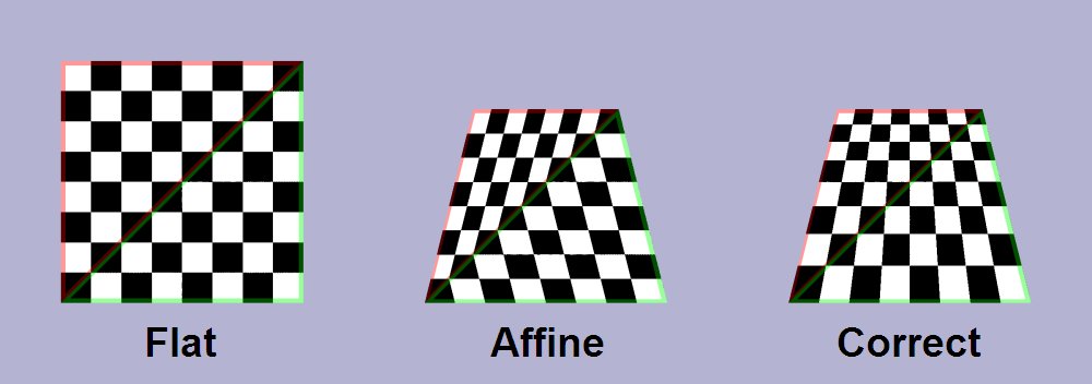
nb = (b2-(b3-b1)*Q-b1)/(x2-(x3-x1)*Q-x1) // Change of b along the x-axis from long to short edge.

In total (ignoring additions and subtractions for now), we have 12 divisions and 5 multiplications (note that the result of the bottom half of the n* formula remains constant and only has to be calculated once.) As dividers and multipliers are pretty expensive in hardware, let's just use one of each, and just iterate through each of the calculations. Using some multiplexers and demultiplexers, we get something like this:

The devil is in the details, as always. Assuming all these wires have registers on them to hold the values, this setup will mostly work. Except for one small thing: the divider is incredibly slow. I just use the Xilinx CoreGen to create a divider unit for me, so that's where I'll get my restrictions, but this should apply to most divider implementations. While the divider can take and calculate new values every clock cycle, it doesn't immediately output the results. With my parameters, it takes no fewer than 32 cycles to produce an output!

As something of a motto in GPUs, latency (the time between input and the corresponding output) isn't important, throughput (how much data we can output every second) is. But we'll still have to deal with this massive latency in the divider, because we can't afford to just wait 32 cycles for every division, not to mention the second division we'll have to do for the n-values. Instead of waiting, we'll just start the calculations for the next triangle. Then, when the divisions are finally done, we'll continue processing the first triangle.

This pipelining, as it's called, is a very efficient way of using those cycles you'd otherwise just be waiting. However, this does mean we'll have to buffer the values for all the triangles we're currently processing. This can be done effectively using shift-registers. Whenever we've calculated everything we can with our current data, we'll shift new data into the registers. Then, when the divider is done, and we're ready for the next step we'll only have to look in the correct position of the shift register to get the original input data that belongs to that triangle.

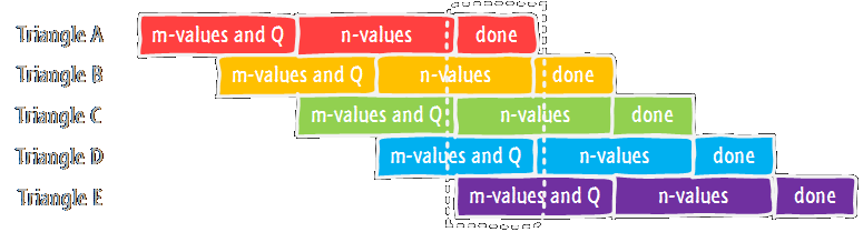
Adding some clock cycles for delays and getting new input and output, I ended up with a processing cycle of 16 clock cycles. In total, the timeline looks a bit like this:

For each triangle, we first calculate the m-values and the Q, wait a bit for the results, then calculate the n-values, wait again, and finally collect the results and push them to the output. Thanks to pipelining, we can start processing the next triangle while waiting for the results of the previous. The dotted box shows what the actual PreCalc block is doing in each processing cycle: calculating the m-values and Q of the current triangle (n), waiting for the results of the previous (n-1), calculating the n-values of triangle n-2, waiting for triangle n-3, and sending triangle n-4 to the output.

All these operations are being done simultaneously (or at least within the same processing cycle) on that one divider and multiplier. In total, we need to hold the data for 5 different triangles, so that's the length of the shift registers. Add some muxes and demuxes, and a little controller to manage this schedule, and we've basically got our PreCalc unit! In total, this means that processing a triangle takes 5 processing cycles of 16 clock cycles each (80 clock cycles), and we can output a new triangle every processing cycle, for a total throughput of 6.25 million triangles per second at a 100MHz clock.

I've fixed most of the drawing pipeline now. A few sorting issues, and poor handling of triangles with a flat top were causing the glitches I saw before. Now just a few off-by-one errors in the final drawing stage it seems.

Just for you guys, I've made a little spinning animation (no projection yet though):

As the deadline for the Hackaday Prize is fast approaching, I thought I'd give you all a quick update on the current status of the project.

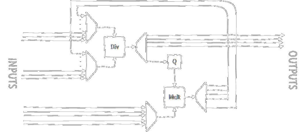
This here is the overall block diagram:

A bit bigger than the one we've been building in the project logs so far, but not much more complicated. Starting from the back, I've made the VGA output an explicit component. I've added an additional scanline buffer, the UV-Buffer, which stores higher precision values for R, G and B, which are processed by the Shader as either high-precision colours, or as UV-coordinates for texture mapping. Textures will of course need some amount of caching, and to save on bandwidth, I'm applying Texture Compression (a derivative of DXT1). On the drawing side not much has changed, just the addition of a Z-Buffer. Triangle input will be passed through memory (for which we need a memory controller).

I'm basically using the memory as a big triangle sorter. Rather than demanding the processor to sort all triangles, triangles are placed into "buckets" in memory, each bucket storing triangles with the same top Y-coordinate. QuickSilver then reads each bucket one by one.

A quick overview of the current status:

Currently I'm cleaning up the drawing pipeling, from PreCalc to Drawline, where there were still some issues. I think you'll like my debug image ;)

The links to Github and an early Wiki are now available.

I'm still working out how best to upload a Xilinx ISE project to Git, so bear with me while I figure it out.

Github: https://github.com/HeavyPixels/QuickSilverNEO

Wiki: http://heavypixels.com/wiki/QuickSilver

In the last log I talked about the basic calculations behind triangle rasterization. But we ended up with a few interpolations (and therefore, divisions) we needed to do every scanline. These are costly in both time and resources, so I want to avoid doing those, or at least try to do them only once per triangle.

One of the main reasons why triangles are used to render 3D graphics is their mathematical unambiguity. For every three points in space,there is exactly one triangle. What's more, a triangle is always flat, unlike quadrangles which can be folded along a diagonal. We can extend this flat surface to get a plane. In essence, the surface of the triangle is a small cut-out of that infinite plane.

There is another way to define a plane: using two vectors and a base point. And no matter where you are on the plane, those two vectors remain the same. So why not use those vectors to define the surface of our triangle?

We're actually already using three of those vectors in a slightly different form: our gradients. The combination of m1, m2 or m3 with the corresponding gradients for the z-axis or colour components gives us the vectors along the edges of the triangle. To make calculation a bit simpler, we would like one the vectors to point along the scanline, so we can calculate the horizontal gradient from that (our n-values before).

I ended up using the following values:

The m1, m2 and m3 values remain the same, as they are used to define the edges of the triangle.

For mz, mr, mg and mb, the vertical gradients for the z-axis and each colour component, I will use the values along the same edge as m1, the edge that goes from the top-most to bottom-most vertex, so we can keep using them for the entire triangle as we descend along that edge.

The horizontal gradients nz, nr, ng and nb will require a bit more work. I will calculate the vector on the widest part of the triangle (along a scanline), the height of the middle vertex (x2, y2). With some mathematical acrobatics I ended up with the following formula for each component c:

nc = (c2-(c3-c1)*Q-c1)/(x2-(x3-x1)*Q-x1)

Where Q is

Q = (y2-y1)/(y3-y1)

Now we only have to calculate the gradients, both vertical and horizontal, one per triangle.

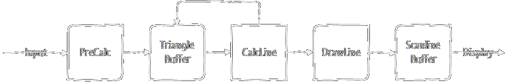
I'll put this in a block called 'PreCalc', for pre-calculation. In the block diagram I've also split the drawing of each scanline into two: CalcLine, which calculates the values along the edges, and DrawLine, which fills the pixels in between.

Although there are other methods for drawing triangles (such as using Barycentric Coordinates, popular in modern GPUs) we'll keep it to just the simplest one: Scanline conversion. In it, a triangle is drawn line-by-line, top-to-bottom, for each scanline on the screen. While its not used in any modern GPU from the last decade and a half, it does have some advantages:

• it's easy to figure out where to start and stop drawing
• very few multiplications and divisions (expensive in hardware)
• little to no overdraw (calculating pixels outside of the triangle)
• neat ordering from top to bottom (useful for QuickSilver's per-scanline rendering)

For these reasons, it was also very popular for old software rasterizers. I learned a lot from a series of articles about such a software renderer by Chris Hecker (creator of SpyParty) published in Game Developer Magazine in '95-'96, and now available on his website (http://chrishecker.com/Miscellaneous_Technical_Articles). As I just want things to be simple and fast, I'll be doing a bunch of things mentioned as "big no-no's" by Chris.

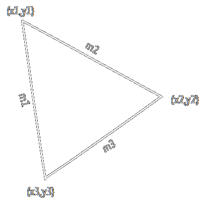
Anyway, the algorithm:

We start by sorting the vertices of the triangle top to bottom: (x1,y1), (x2,y2) and (x3,y3). We then calculate the gradients of the lines connecting the vertices, which we'll call m1, m2 and m3:

Next, we'll take to variables, xa and xb, which we'll use to walk along the edges of the triangle. Both will start at the top, at x1. xa will walk along the line from (x1,y1) to (x3,y3) using m1, and xb will walk along the line from (x1,y1) to (x2,y2) using m2.

Each scanline we just add the gradient value to xa and xb, and draw a line between them. When we reach reach y2, we switch to using m3 for xb, which now follows the line from (x2,y2) to (x3,y3). Draw a line for every scanline from y1 to y3 and we have our triangle. Of course, this way the triangle will only be filled with a single colour. The get some more variation, we can apply Gouraud Shading, which interpolates colour components from each vertex along the triangle. Again, we'll calculate a gradient for each edge:

We can then use variables ca and cb to calculate the colour at each point along the edges, like we did with xa and xb. Finally, we need to interpolate between the two edges on each scanline to get the colours in between, using another gradient:

We use the same calculation for each of the three colour components (red, green and blue), and for the z-coordinates (not really accurate, but close enough).

Now, we want to get all of this calculation to happen in hardware, so it's a good idea to summarise the operations we need to perform:

For each triangle:

• 3 divisions for each of x, z, r, g and b (15 in total)
• ... and a bunch of subtractions

For each scanline in that triangle:

• 1 division for each of z, r, g and b (4 in total)
• ... and a bunch of additions and subtractions

And for each pixel in that scanline:

• Just some additions!

Dividers in hardware are big and slow, taking up a lot of space on the FPGA, and taking dozens of cycles to get an answer. So, if at all possible, we want to avoid using them. And if we can't, we should take the time reuse them as much as possible. I'm happy to see that the operations we do most often, the per-pixel operations, are just some additions, which are really cheap in FPGA fabric. We can't really avoid the divisions in the per-triangle operations, but we really only need to execute that once per triangle. Compared to the number of pixels (hundreds of thousands per frame) the triangles are few in number (a couple thousand per frame), so we'll have plenty of time to calculate, and we could do it all with just one divider.

What I am worried about is the per-scanline operations. These will have to happen for every scanline, for every frame, so these could become a major bottleneck without a lot of additional buffering. Plus, I really want to avoid that second divider.

In the next post I'll perform some nasty mathematical hacking that makes Chris Hecker sad, and do away with that darned divider.

In a traditional rendering pipeline, each triangle is drawn individually and completely to a framebuffer. When all triangles are drawn the content of the framebuffer is sent to the display and the triangles for the next frame are rendered.

Unfortunately for QuickSilver, the Nexys 2 simply does not have the memory bandwidth required to render each and every triangle on-screen individually and then load the complete framebuffer for display.

Which is why we're not going to use a framebuffer.

Instead, we're going to send the rendered pixels straight to the display. Unlike a framebuffer, however, a typical display device does not allow random access; the pixels must be written in a certain order: left-to-right, top-to-bottom. And the pixels we send to the display are final, no overwriting allowed. So in order to send a pixel to the screen, we must have first sampled every single triangle that covers this pixel. Which gives us our first requirement:

The information of every single triangle that covers the rendered area must be present at the same time.

Although the Spartan-3E FPGA on the Nexys-2 doesn't have enough space for an entire framebuffer, it can easily fit a few scanlines. That way we don't have render in exact left-to-right order, and we can render an entire line for each triangle, instead of just a single pixel, which helps to reduce overhead. Triangles do tend to be taller than a single scanline, so we'll need to remember the triangle data until it has been fully rendered:

Triangle data must be buffered until the triangle is fully rendered.

With scenes easily containing many thousands of triangles, that buffer needs to be quite large if we store every random triangle in the rendering pipeline, and memory space and bandwidth are exactly the things the Nexys 2 lacks. Fortunately, we can optimise. By sorting the incoming triangles top-to-bottom only the triangles that cover the current scanline need to be stored. Furthermore, if a triangle is found in the buffer that is completely below the current scanline then we can safely skip all triangles that follow. This saves additional overhead for loading and checking each triangle.

Incoming triangle data must be sorted top-to-bottom based on their topmost Y-coordinate.

The scanline rendering architecture is starting to take shape:

• Triangles are sorted based on their topmost Y-coordinate.
• Triangles are stored in a buffer.
• Scanlines are drawn top-to-bottom.
• Triangles are loaded from the buffer and a single scanline is rendered.
• Triangles that have been completely rendered are removed from the buffer.
• If a triangle is found in the buffer that is completely below the current scanline, it and all following triangles are skipped.
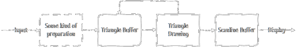
• When the end of the triangle buffer has been reached, the current scanline is complete and is sent to the screen. The next scanline starts rendering.

Scanline rendering differs greatly from traditional framebuffer rendering. This has several advantages, and limitations:

Advantages:

• No Framebuffer. Memory footprint is greatly reduced because of this.
• Guaranteed 60Hz. Everything is sent straight to the screen, so no dropped frames and no tearing.
• Cheaper Z-buffering. We only need a single scanline of Z-buffer, instead of the entire frame.

Disadvantages:

• No Framebuffer. Framebuffer effects, complex alpha, environment mapping and multi-pass rendering are all out.
• Guaranteed 60Hz. Sounds great, but what happens if we go slightly over our render time? It's impossible to slightly delay the frame and take a bit more time to render it. Instead, triangles will be skipped and visual artefacts will be visible. Because everything is rendered per-scanline, triangle density becomes an important factor too.
• Hard triangle limitations. In addition to the timing issues mentioned above, the triangle buffer itself poses a hard limit on the number of triangles that can be rendered on each scanline. In practice, the render time imposes the stricter limit.

In the next post I'll talk a bit about the basic formula behind the triangle rasterization.