I got temporarily obsessed with designing a 3-axis field coil to calibrate the MLX90393 sensor. A 3-axis coil would allow all three axes to be calibrated with the sensor in a single position. This allows for easy detection and compensation of angular errors: not aligning the sensor exactly with the coil axes. In addition, a 3-axis coil would make it easy to register the magnetic coordinate system of the sensor into the spatial coordinate system of the printer - this is sure to be slightly different each time you mount/detach the sensor head.

I started playing with 3-axis Helmholtz designs, but for multi-turn windings, the required spacing makes for a clunky design. Here's one of the mock-ups I was playing with:

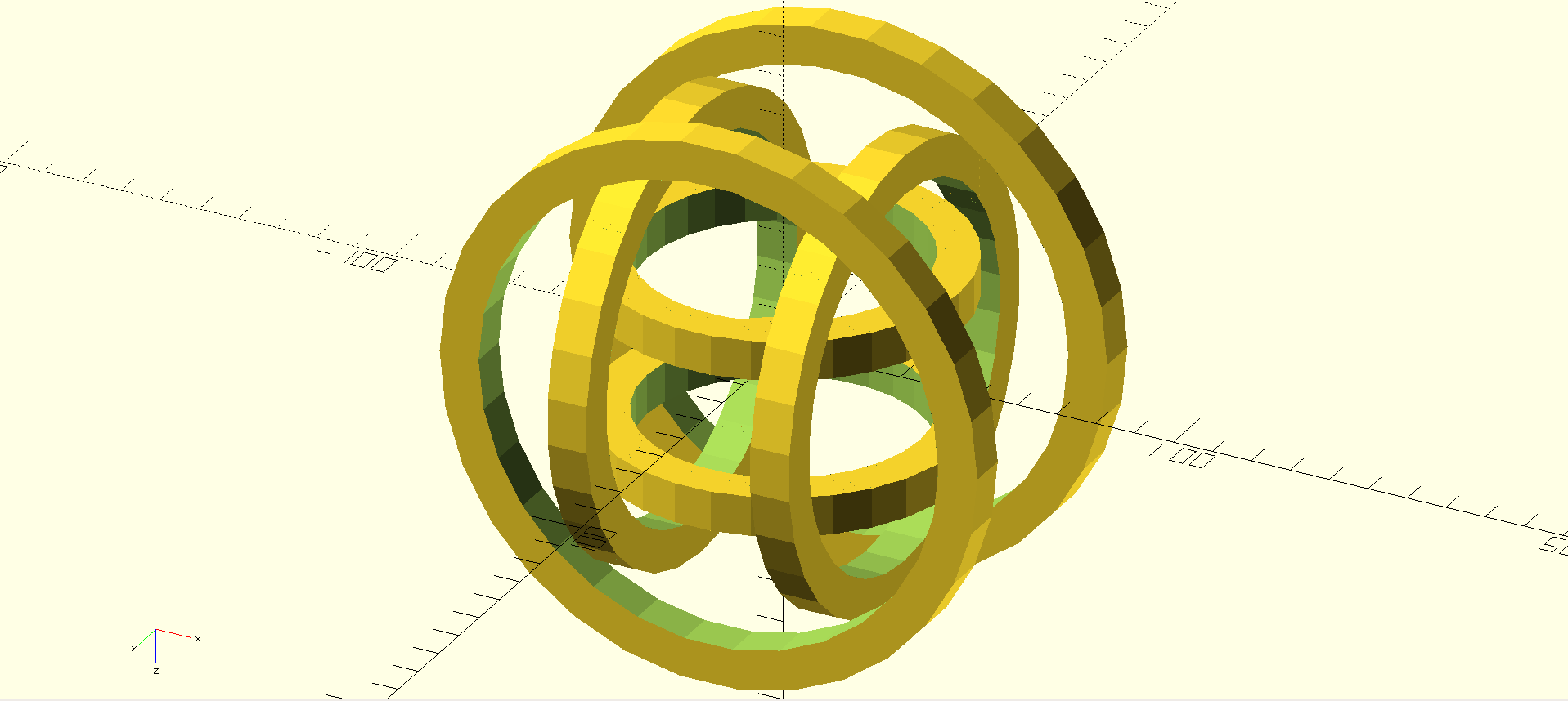
The size of the windings also allows only a very small active volume, and the nested configuration complicates the mechanical design (which I didn't complete). I started to wonder how important the spacing was in the Helmholtz design. If the spacing constraints could be relaxed, I could use something like this:

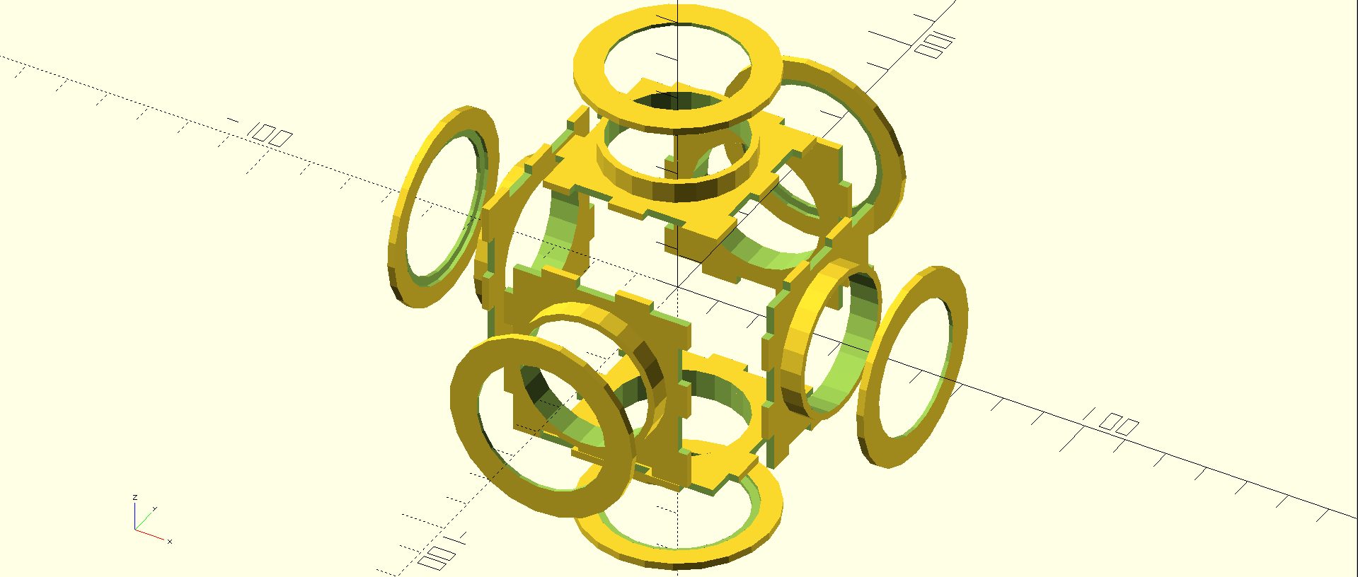
Here, the windings are farther apart than in the Helmholtz design. This allows the windings to be on the cube faces, which are all the same shape, and all the parts can be conveniently printed "flat" on the printer bed. I printed a few of these, and they're fun to snap together (the spool caps have to be glued). Mechanically, this is a win, but I had no idea what this does to the field, so some simulations were in order.

Unfortunately, the math I'd done so far could only calculate the field along the coil axis; the field in the full volume of the coil was unknown. I downloaded some finite-element software ( Elmer, a general-purpose package, and MaxFEM, aimed solely at magnetics) and played around a bit. These are powerful tools with steep learning curves, and while I'm going to keep at it and learn to use them eventually, using them for my immediate needs feels like slicing bread with a chainsaw. So, I decided to write the "bread knife" of field coil design.

I lucked out and found the paper Simple Analytic Expressions for the Magnetic Field of a Circular Current Loop on the NASA Technical Reports server. This paper provides equations for the full vector field surrounding a loop of current, and the equations are fairly simple, in part because the required elliptic integrals are conveniently hidden. To my great joy, I found that the python scipy package contains routines for numerical evaluation of these integrals, greatly simplifying field calculation. Since the field obeys superposition, these equations can be used to calculate the field surrounding any 3D configuration of circular current loops - which covers just about any coil I might think of using. I was able to create the core of a python simulation fairly quickly; it's less than 100 lines of code. Having the simulation as a library is very convenient - you can program all sorts of analyses and what-if's easily.

Here's the model for the "filamentary" current loops simulated:

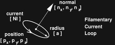
The loop is assumed to be a conductor of infinitesimal diameter, centered in 3-space at position p, of radius a, with normal n, and carrying a magnetizing current NI. For normal "magnet wire" in relatively large loops, this model will work very well.

The "loopfield" code is here on GitHub, as well as on PiPY ('pip install loopfield' gets you a copy, but check out the examples on GitHub). It requires matplotlib for the plotting functions, but the core engine just uses numpy and scipy. Usage is very easy - here's code to calculate the vector field for a single-turn coil:

#!/usr/bin/env python3
import loopfield as lf
# create empty field with specified units
field = lf.Field(length_units = lf.cm,
                 current_units = lf.A,
                 field_units = lf.uT)
# single-turn 10 cm x-oriented coil at origin
position = [0., 0., 0.]
normal = [1., 0., 0.]
radius = 10.
current = 1.
c = lf.Loop(position, normal, radius, current)
# add loop to field
field.addLoop(c);
# evaluate vector field at origin
B = field.evaluate([0., 0., 0.])
print('B = ', B)

You can add more loops and evaluate the field at more points as required. The package will also plot a 2-d slice of the field, with field lines, colored areas based on user-supplied criteria, and simple volume annotations. There appears to be a bug in the streamplot function of the matplotlib python package which would crash occasionally producing these plots. I made a temporary fix (aka quick hack) in my local matplotlib, and will submit an official patch once I figure out how to fix it properly.

I started with modelling the coils I had already wound. Here's the Helmholtz coil, simulated with two loops in place of the multi-turn windings. The field at the center of the coil agrees with earlier calculations. The red region represents the volume in which the x-component of the field is within 1% of the central value; it shows the well-known "octopus" shape. I added a hand-tuned circle of radius 12.5mm to illustrate that the usable volume (at 1% error tolerance) encloses a 25mm diameter sphere in the center of the coil. The field is sampled at 101 x 101 points to generate this plot, which takes about five seconds to compute on my desktop.

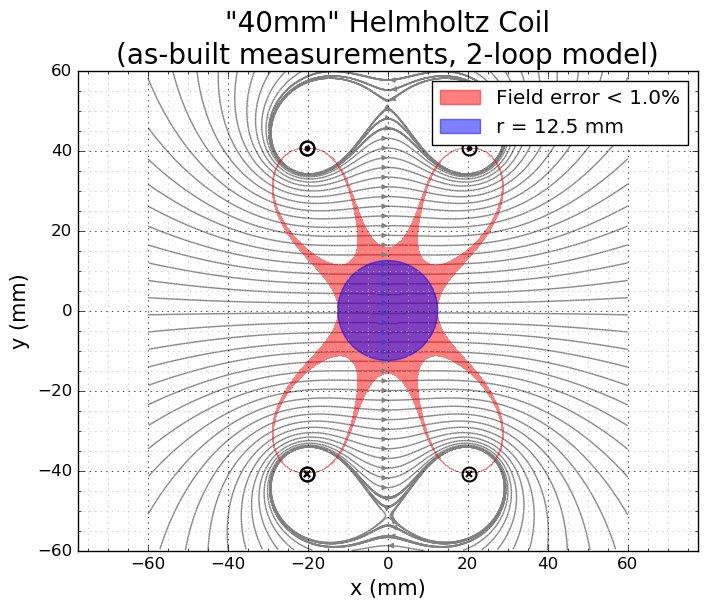
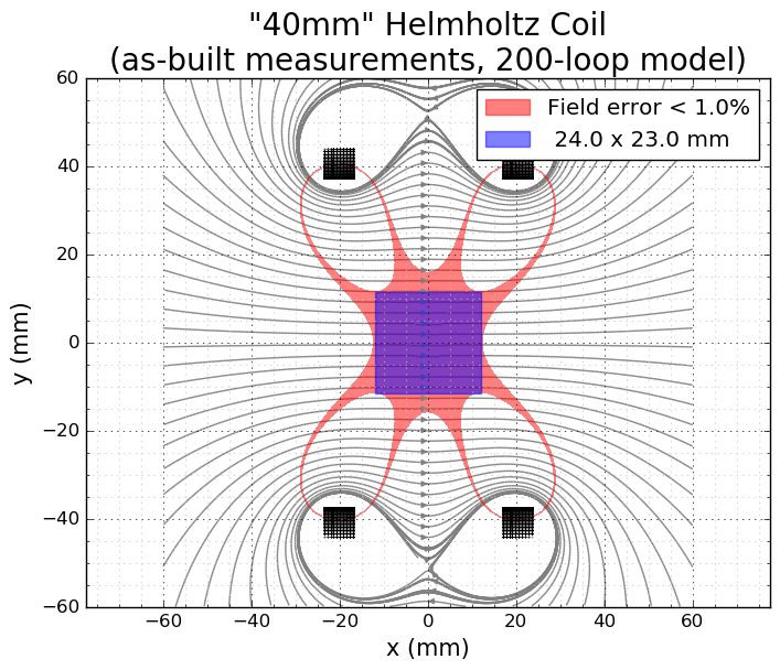
When I simulated this coil before, I had questions about how the "large" windings affected the field. Here's the answer - I modeled the actual 100 loops per winding with the same as-built measurements I had for the simple wxMaxima calculations. This calculation (again using 101 x 101 field samples) takes a little over a minute to compute. I used a rectangular annotation, since positioning errors for the probe along the three axes are likely to be relatively uncorrelated (the error region will be square, not circular). Other than my choice of different annotations, the 1%-tolerance regions are nearly identical, showing that the "large" windings are not producing significant error.

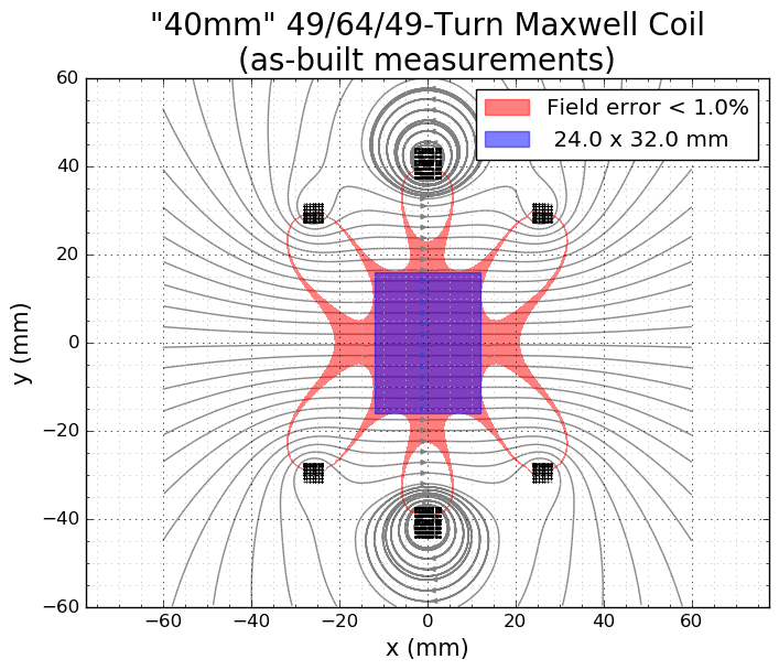
While I was at it, I simulated the original Maxwell coil I had wound. The sub-1%-error region is indeed larger than the Helmholtz design and exhibits a [insert 12-armed animal name] shape.

Cube-Coil Fail

Oh, I almost forgot why I wrote this simulator. I wanted to see what the effect moving the windings out to the cube faces had on the field. Simulating just one axis of the coil (we could do all three here), we get the following:

The blue region is the same size as the one on the Helmholtz design above - and the coil radius is identical. That Helmholtz dude knew what (tf) he was doing! Clearly, this coil design is a bust, despite the nice mechanical properties. I'll have to come up with another one. At least now I have a tool to evaluate them.

Other Uses

While these plots (and the loopfield.plot module) are all in 2D, the core of the code calculates the field in 3D. This brings me to the other reason I wanted to write this simulator - I can use it to generate simulated scan data. With a little more code, I can write out simulated 3D scans for fields around various coils, then compare the simulations with actual data from the scanner. This will provide a way to check the scanning error.

Next Up

I have a few experiments to do with the MLX90393 to check temperature calibration and accuracy on the second part I have wired up. I'm also making some decent progress on the scanning and viewing software so I should be able to crank out a few interesting test scans in the next few days.

ADDENDUM (7/7/2016)

I tried installing the loopfield python package on an older linux distro, and ran into some trouble. Here's a recipe for installing it and the required dependencies in a python3 virtualenv, so it doesn't conflict with the python modules installed by the package manager. It was tested in a Linux Mint distro, so you may have to install different packages for different distros:

# you need to be able to compile FORTRAN code to install scipy
# and have the lapack and blas system libraries installed
apt-get install python3-dev
apt-get install python-virtualenv
apt-get install libblas-dev
apt-get install liblapack-dev
apt-get install gfortran
# create a virtual python environment to install into
virtualenv -p python3 LF
# enter the environment (you need to do this in every shell)
source LF/bin/activate
# install loopfield and all the dependencies
pip install loopfield

that last line takes a *long* time to run, having to compile a lot of FORTRAN code. It also prints what appear to be compile error messages to the screen as it compiles scipy, but in the end, reports that everything was installed, and it runs fine.

The patch for matplotlib can be applied as follows:

patch -p0 <<EOF 
--- LF/lib/python3.4/site-packages/matplotlib/streamplot.py 2016-07-07 09:32:47.000000000 -0400
+++ LF/lib/python3.4/site-packages/matplotlib/streamplot_patch.py 2016-07-07 10:35:22.911117920 -0400
@@ -368,7 +368,9 @@
                 self._mask[ym, xm] = 1
                 self._current_xy = (xm, ym)
             else:
-                raise InvalidIndexError
+                #raise InvalidIndexError
+                pass
+
 
 
 class InvalidIndexError(Exception):
EOF

The matplotlib streamplot() function I use to render field lines uses the efficient python exception handling mechanism to implement backtracking when calculating field lines. It's a nice technique I've seen elsewhere, but in this case it looks like there's a codepath which doesn't handle the exception, so it gets passed all the way up to us.