 hanno
hanno-
Solving the Math: Computing the Servo Angles
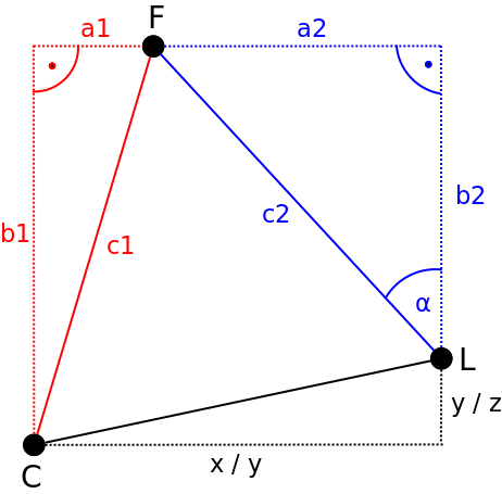
08/15/2016 at 08:23 • 0 commentsAfter the pixel position and size of a face in the camera image has been detected, the horizontal and vertical servo motor angles can be computed in order to point the air flow into the direction of the face. The geometric relationships between the camera C, the fan L and the face F can be drawn (either for top or side view) in the following way:
As can be seen the angle α represents the servo motor angle for pointing either the horizontal or![]()
vertical air flow (depending on looking from either the top or the side) into the direction of the face. By exploiting the two additional triangles drawn in red and blue, one can apply some simple trigonometric computations to derive the servo motor angle α.
Computing the distance to the face (c1)
In order to compute the distance to the face c1 in a camera image one first needs to determine the focal length F of the camera.
Determining the focal length F of the camera
Assuming a pinhole camera model, the focal length F can be obtained by recording an object with a known width W with a distance D with the camera. After determining the apparent width of the object in pixels P, one can compute the perceived focal length F of the camera according to the following formula:
E.g. if we place a ball with a diameter/width W=10 cm and a distance D=100 cm in front of our camera and measure an apparent width of the ball in pixels P=20, then the focal length of our camera is:
Please note: As the horizontal and vertical focal lengths of the camera f_x and f_y are already contained in the camera matrix obtain from using OpenCVs camera calibration tool, one can simply use them instead of performing the calibration procedure outlined above.
After having obtained the focal length F the distance to the face c1 can be computed using triangle similiarity:
Finding the distance to a face c1 using triangle similarity
Assuming we have found the focal length F of our camera in the previous step, we can now compute the distance c1 to an object (e.g. a face) with a known width W using the so-called triangle similarity:
As an example, I will assume the average width of a face is W=14 cm. If a face has been detected in the camera image and and the apparent width of the face in pixels is P=25, the distance to the face can be computed by taking the focal length F of the camera into account:
Hence, the distance c1 to the face is 112 cm.
Determining the distance of the face from the center optical axis (a1)
After having determined c1 the distance of the face from the center optical axis a1 of the camera can be computed. Assuming an average width of a face W in cm, the width in pixel of the face detected in the camera image P and the position of the center of our face in pixel C, one can compute a1 according to the following formula:
where i represents the horizontal (or respectively vertical) resolution of the camera image in pixels. w corresponds to the width of the bounding box surrounding the face in pixels obtained from the face recognition algorithm.
Determining the servo motor angle α
After having determined c1 and a1 in the red triangle the servo angle α can be derived from simple Pythagorean equations. The corresponding formulas for determining the horizontal servo angle are shown below:
After having calculated the lengths a2, b2 and c2 of the blue triangle the servo motor angle α can now be determined by the following formula:
The FaceToPosition Class
The calculations described above are implemented in the FaceToPosition class. Once instanced the corresponding object takes the width of the face, the position of the bounding box around the face and the focal lengths of the camera lens into account in order to estimate the position of the face relative to the camera and computes the relative servo angles for the horizontal and vertical lamellae of the fan accordingly. The following video shows the code in action:
The code is available via my GitHub repository.
-
Face Detection using a Haar Cascade Classifier
07/14/2016 at 15:20 • 1 commentAfter correction for lens distortions in the camera images, I apply a face detection algorithm on each camera image to obtain the apparent pixel position as well as the apparent pixel width and height of a face in front of the camera. For this purpose I make use of a set of haar-like features trained to match certain features of image recordings of frontal faces. I then use a classifier which tries to match the features contained in the haar feature database with the camera images in order to detect a face (see Viola-Jones object detection). It is notable, that although training a set of haar-filters of facial features is in principle possible (given a large enough database with images of faces), in the scope of this project I use a bank of pre-trained haar-like features that already comes with OpenCV.
Detecting facial features using haar-like features
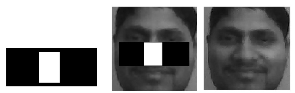
Haar-like features can be defined as the difference of the sum of pixels of areas inside a rectangle, which can be at any position and scale within the original image. Hence, by trying to match each feature (at different scales) in the database with different positions in the original image the existence or absence of certain characteristics at the image position can be obtained. These characteristics can be for example edges or changes in textures. Hence, when applying a set of haar-like features pre-trained to match certain characteristics of facial features, the correlation by which a certain feature matches an image feature can tell something about the existence or non-existence of certain facial characteristics at a certain position. As an example, in the following figure a haar-like feature that looks similar to the bridge of the nose is applied onto a face (image taken from Wikipedia):
![]()
In order to detect a face using haar-like facial features one can use a cascade classifier. Explaining the inner workings of the cascade classifier used here is out of the scope of this project update. However, this video by Adam Harvey gives quite an intuitive impression of how it works:
OpenCV Face Detection: Visualized from Adam Harvey on Vimeo.
Face detection using haar-like features using a cascade classifier can be implemented in OpenCV in the following way:
import cv2 from matplotlib import pyplot as plt # Initialize cascade classifier with pre-trained haar-like facial features classifier = cv2.CascadeClassifier("haarcascade_frontalface_alt2.xml") # Read an example image image = cv2.imread("images/merkel_small.jpg") # Convert image to grayscale gray = cv2.cvtColor(image, cv2.COLOR_BGR2GRAY) # Detect faces in the image face = classifier.detectMultiScale( gray, scaleFactor=1.1, minNeighbors=5, minSize=(30, 30), flags = (cv2.cv.CV_HAAR_SCALE_IMAGE + cv2.cv.CV_HAAR_DO_CANNY_PRUNING + cv2.cv.CV_HAAR_FIND_BIGGEST_OBJECT + cv2.cv.CV_HAAR_DO_ROUGH_SEARCH) ) # Draw a rectangle around the faces for (x, y, w, h) in face: cv2.rectangle(gray, (x, y), (x+w, y+h), (0, 255, 0), 2) # Display image plt.imshow(gray, 'gray')![]()
Here I first initialize a cascade classifier object with a pre-trained database of haar-like facial features (haarcascade_frontalface_alt2.xml) using OpenCVs CascadeClassifier class. The cascade classfier can then be used to detect facial features in an example image using its detectMultiscale method. The method takes the arguments scaleFactor, minNeighbours and minSize as an input.
The argument scaleFactor determines the factor by which the detection window of the classifier is scaled down per detection pass (see video above). A factor of 1.1 corresponds to an increase of 10%. Hence, increasing the scale factor increases performance, as the number of detection passes is reduced. However, as a consequence the reliability by which a face is detected is reduced.
The argument minNeighbor determines the minimum number of neighboring facial features that need to be present to indicate the detection of a face by the classifier. Decreasing the factor increases the amount of false positive detections. Increasing the factor might lead to missing faces in the image. The argument seems to have no influence on the performance of the algorithm.
The argument minSize determines the minimum size of the detection window in pixels. Increasing the minimum detection window increases performance. However, smaller faces are going to be missed then. In the scope of this project however a relatively big detection window can be used, as the user is sitting directly in front of the camera.
Further, several flags are passed to the classifier. These are: a) CV_HAAR_SCALE_IMAGE, b) CV_HAAR_DO_CANNY_PRUNING, c) CV_HAAR_FIND_BIGGEST_OBJECT and d) CV_HAAR_DO_ROUGH_SEARCH.
The flag CV_HAAR_SCALE_IMAGE tells the classifier that haar-like features are applied on image data, which is what we are doing for detecting faces.
The flag CV_HAAR_DO_CANNY_PRUNING is useful when detecting faces in image data, as it tells the classifier to skip sharp edges. Hence, the reliabilty by which a face can be detected is increased. Depending on the backdrop, performance of the algorithm is increased when passing this flag.
The flag CV_HAAR_FIND_BIGGEST_OBJECT sets the classifier to only return the biggest object detected. Whereas the flag CV_HAAR_DO_ROUGH_SEARCH sets the classifier to stop after a face has been detected. Setting both flags drastically improves performance, when only one face needs to be detected by the algorithm.
When a face has been detected by the classifier it returns a list containing the lower left pixel position (x,y) and the width and height (w,h) of a bounding box surrounding the face. These parameters can then (hopefully!!) be used to determine the position of the face in the camera in order to control the servo motor angles.
The FaceDetection class
In order to detect faces from the unwarped camera images i wrote a Python class which implements face detection using haar-like features as described above. The class is implemented as a Python multiprocessing task and takes the unwarped camera images as an input. As an output it returns the x,y coordinates and the size of the bounding box of the face. Unfortunately, the x,y coordinates obtained from OpenCV's cascade classifier jitter over time. This will result in jittery movements of the fan's lammelae when directly computing servo angles from the ccordinates of the face in the image. Hence, I implemented a temporal first-order lowpass filter which removes high frequency oscillations from the face coordinates over time. The following video shows a short test of the face detection module:
-
Correcting for Lens Distortions
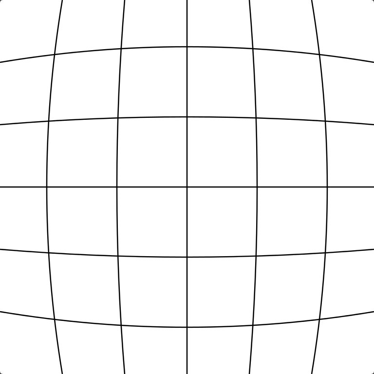
07/12/2016 at 11:41 • 3 commentsCertain types of camera lenses (such as in the webcam used in this project) introduce distortion characteristics to the images such that objects along the optical axis of the lens occupy disproportionately large areas of the image. Objects near the periphery occupy a smaller area of the image. The following figure illustrates this effect:
![]()
This so-called barrel distortion results in the fact that the representation of distance relations in the real world is not the same as in the camera image -- i.e. distance relations in the camera image are non-linear.
However, in this project, linear distance relations are required to estimate the servo motor angles from the camera images. Hence, lens distortions have to be corrected by remapping the camera images to a rectilinear representation. This procedure is also called unwarping. To correct for lens distortions in the camera images I made use of OpenCV's camera calibration tool.
Estimation of lens parameters using OpenCV
For unwarping images OpenCV takes the radial and the tangential distortion factors into account. Radial distortion is pretty much what leads to the barrel or fisheye effect described above. Whereas, tangential distortion describes the decentering of the optical axis of the lens in accordance to the image plane.
To correct for radial distortion the following formulas can be used:
So a pixel position (x, y) in the original image will be remapped to the pixel position (x_{corrected}, y_{corrected}) in the new image.
Tangential distortion can be corrected via the formulas:
Hence we have five distortion parameters which in OpenCV are presented as one row matrix with five columns:
For the unit conversion OpenCV uses the following formula:
The parameters are f_x and f_y (camera focal lengths) and (c_x, c_y) which are the optical centers expressed in pixels coordinates. The matrix containing these four parameters is referred to as the camera matrix.
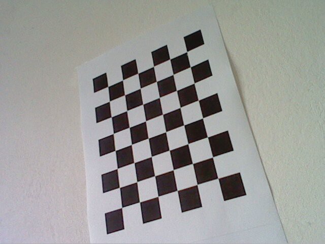
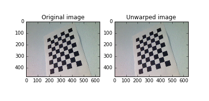
The camera matrix as well as the vector containing the distortion coefficients can be obtained by using OpenCVs camera calibration toolbox. OpenCV determines the constants in these two matrices by performing basic geometrical equations on several camera snapshots of calibration objects. For calibration I used snapshots of a black-white chessboard pattern with known dimensions taken with my webcam:
To obtain the camera matrix and the distortion coefficients I used the calibrate.py script which comes with OpenCV (see 'samples' folder). The script is basically a wrapper around OpenCVs camera calibration functionality and takes several snapshots from the calibration object as an input. After having run the script by issuing the following command in a shell![]()
python calibrate.py "calibration_samples/image_*.jpg"the calibration parameters for our camera, namely the root-mean-square error (RMS) of our parameter estimation, the camera matrix and the distortion coefficients can be obtained:RMS: 0.171988082483 camera matrix: [[ 611.18384754 0. 515.31108992] [ 0. 611.06728767 402.07541332] [ 0. 0. 1. ]] distortion coefficients: [-0.36824145 0.2848545 0.00079123 0.00064924 -0.16345661]Unwarping the images
To unwarp an image and hence correct for lens distortions I made use of the recently acquired parameters and OpenCVs remap function as shown in the example code below:
import numpy as np import cv2 from matplotlib import pyplot as plt # Define camera matrix K K = np.array([[673.9683892, 0., 343.68638231], [0., 676.08466459, 245.31865398], [0., 0., 1.]]) # Define distortion coefficients d d = np.array([5.44787247e-02, 1.23043244e-01, -4.52559581e-04, 5.47011732e-03, -6.83110234e-01]) # Read an example image and acquire its size img = cv2.imread("calibration_samples/2016-07-13-124020.jpg") h, w = img.shape[:2] # Generate new camera matrix from parameters newcameramatrix, roi = cv2.getOptimalNewCameraMatrix(K, d, (w,h), 0) # Generate look-up tables for remapping the camera image mapx, mapy = cv2.initUndistortRectifyMap(K, d, None, newcameramatrix, (w, h), 5) # Remap the original image to a new image newimg = cv2.remap(img, mapx, mapy, cv2.INTER_LINEAR) # Display old and new image fig, (oldimg_ax, newimg_ax) = plt.subplots(1, 2) oldimg_ax.imshow(img) oldimg_ax.set_title('Original image') newimg_ax.imshow(newimg) newimg_ax.set_title('Unwarped image') plt.show()![]()
Here, after generating an optimized camera matrix by passing the distortion coefficients d and the camera matrix k into OpenCV's getOptimalNewCameraMatrix method, I generate the look-up-tables (LUTs) mapx and mapy for remapping pixel values in the original camera image into an undistorted camera image using the initUndistortRectify method.
Each of the two LUTs represent a two-dimensional matrix LUT_{m,n} where m and n represent the pixel positions of the undistorted image. The LUTs mapx and mapy at the positions (m,n) contain the pixel coordinate x or respectively y in the original image. Hence, I construct an undistorted image from the orginal image, by filling in the pixel value at the respective position (m,n) in the undistorted image using the pixel value at position (x,y) in the original image. This is performed using OpenCV's remap method. As the pixel positions (x,y) specified by the LUTs do not necessarily have to be integers, one has to define an algorithm for interpolating a pixel value from non-integer pixel positions in the original image. Here I use a simple bilinear interpolation specified by the argument INTER_LINEAR which gets passed in the remap method.
The Unwarping class
In order to unwarp the images obtained from the webcam, I have written a Python class, which performs the computations as described above (see Github repository). Same as in the class for controlling the servos, I use Python's multiprocessing library which provides an interface for forking the image unwarping object as a separate process on one of the Raspberry Pi 2's CPU cores.
-
Controlling the Servos
07/11/2016 at 20:03 • 0 commentsDue to job and family obligations I was only able to work occasionally on the project. However, I finished the servo control via the Raspberry Pi:
For controlling the servos via the Raspberry Pi I decided to use Richard Hirst's excellent ServoBlaster driver. After installation (requires Cython and Numpy) it creates a
/dev/servoblaster
device file in the Linux file system, allowing the user to generate a PWM signal on one (or several) of the Raspberry Pi's GPIO pins. Controlling the servos is as easy as echoing the desired pin and pulse width to the driver:
echo 3=120 > /dev/servoblasterIn the example above a pulse width of 120ms is set on GPIO pin 3.Multithreading
Based on the device driver I wrote a Python class (see 'servo_control/ServoControl' on GitHub) in order to control the servos from within my software framework. As the Raspberry Pi 2 has four CPU cores and the face detection part is computationally quite demanding, I implemented the class to run as a multiprocessing subprocess. This allows to efficiently leverage the multiple CPU cores on the Raspberry Pi 2 by spawning different tasks (e.g. face detection, servo control,...) on the different cores. In order to exchange data between the different processes I decided to use Sturla Molden's sharedmem-numpy library. Python's multiprocessing library allows for sharing memory between processes using either Values or Arrays. However, as I would like to pass camera images stored as Numpy arrays between the processes later on, using sharedmem-numpy currently seems to be the way to go. Although the author states that the library is not functional on Linux and Mac it seems to work quite well on the Raspberry Pi running Raspbian Jessie. However, I had to write a small patch to make things
work (can be found in the project's GitHub repo).
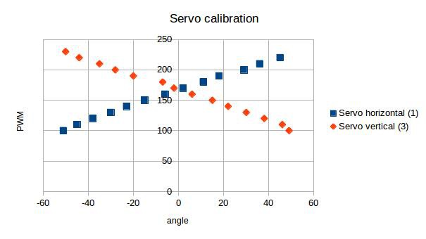
Servo calibrationIn order to set the servo motors to a specific angle, the angle has to be remapped to a corresponding pulse width. By measuring the angle for the horizontal and vertical lamellae at different pulse widths using a triangle ruler, I found that the transfer function is almost linear:
![]()
Hence, the transfer function for remapping a specific servo motor angle α to a specific pulse width p can be estimated by fitting a simple linear regression to the dataset
where m is the slope and b the intercept at the y-axis. I used LibreOffice Calc to do so (see calibration.ods in GitHub repo).
Low-pass filtering of input values
The speed of servo movement is controlled by stepwise incrementing or decrementing the pulse width of the servos at a defined frequency (currently 100Hz) until a desired angle has been reached. To smoothen overall servo movement and to avoid possible problems with jittery input signals, I implemented a temporal low-pass filter in between the computation of input angles and output pulse width. I will see how this works out when face detection is implemented. So, next step will be to hook up a webcam and get face detection running using OpenCV...
-
The Mechanical Prototype
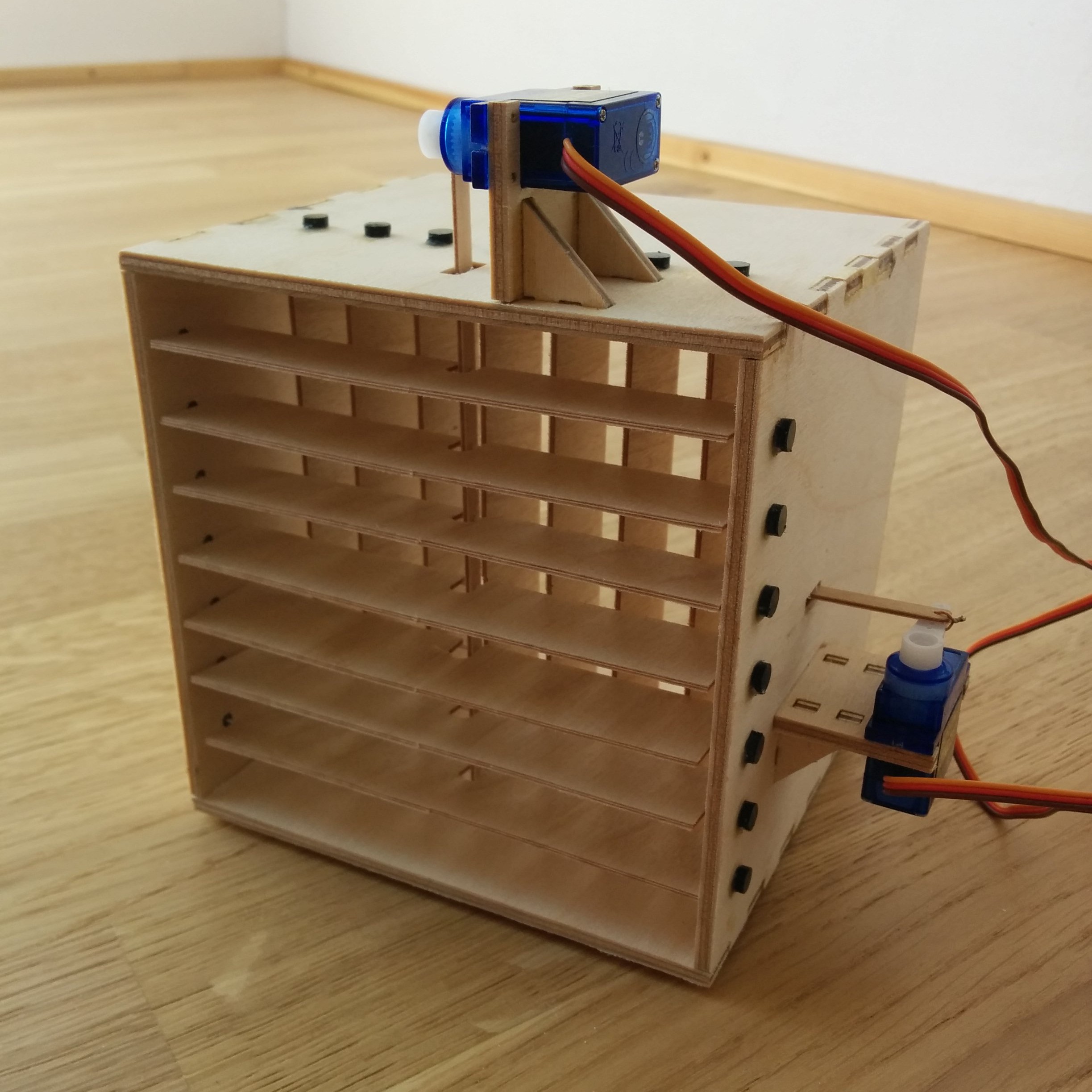
06/26/2016 at 11:21 • 0 commentsHaving designed the mechanical prototype using FreeCad, I finished building and assembling the hardware during the last two days. I have milled the fan's casing, servo parts and the lamellae from birch plywood using my CNC router. The bearings for holding the lamellae in place were milled from POM (Acetal). All parts are available via my GitHub account. Although my first intention was to build the whole device from acrylic glass I found it much cheaper and more convenient to build the first prototype from wood. After cutting the glass fiber rods I assembled everything using (a lot of) superglue:
![Front of mechanical hardware assembled]()
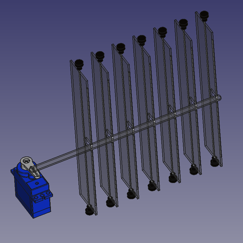
As can be seen from the image above and the screenshot below, the mechanical setup is really simple. The horizontal and vertical lamellae are connected to the corresponding servo motors. Hence, the servos linearily control either the horizontal or vertical direction of air flow.
![]()
In order to test the mechanics, I hooked up the servos to a spare RC receiver controlling the servos via an RC remote. The mechanics seem to work really well. I will upload a video soon.
Next step will be to hook up the servos to the Raspberry Pi and start coding...
AutoFan - Automated Control of Air Flow
Avoiding fatigue by automatically controlling the direction of a fan's air flow using face and eye blink detection.
