-
Racing the Beam Ray Tracer
12/02/2018 at 05:17 • 0 commentsOriginally published here: https://tomverbeure.github.io/rtl/2018/11/26/Racing-the-Beam-Ray-Tracer.html
Executive Summary
- This project uses real-time ray tracing to render a bouncing sphere on a plane.
- Think of it as a technology demo, the way they were made in the late eighties and early nineties for Amiga, PCs, Commodore 64 etc.
- The techique used is entirely NOT scalable and thus kind of useless. It can’t be used for anything that has more than a handful of objects.
- Everything is done using limited precision floating-point. The parameterizable floating-point library stands on its own and should be useful for anyone who needs to issue one operation per clock but doesn’t really care about pipeline latency.
- Everything is written in SpinalHDL.
https://player.vimeo.com/video/303938705
Table of Contents
- Introduction
- The HW Platform
- Racing the Beam - Graphics without a Frame Buffer
- One Pixel per Clock Ray Tracing
- A Floating Point C model
- From Floating Point to Fixed Point
- Math Resource Usage Statistics
- Scene Math Optimization
- Start Your SpinalHDL RTL Coding Engines! Or… ?
- Conversion to 20-bit Floating Point Numbers
- Building the Pipeline
- SpinalHDL LatencyAnalysis Life Saver - Automatic Latency Matching
- Progression to C Model Match
- Intermediate FPGA Synthesis Stats - A Pleasant Surprise!
- A Sphere Casting a Shadow and a Directional Light
- SpinalHDL - Selectively Using HW Multipliers
- Camera Movement and Flexibility - Bringing in a CPU
- Final Toplevel Pipeline
- Text Overlay - The Final Step
- Total Resource Usage and Critical Path
- The End
Introduction
One of the most exciting moments of a chip designer is the first power-on of freshly baked silicon. Engineers have been flown in from all over the world. Debug stations are ready. Emails are being sent with hourly status updates: “Chips are in SFO and being processed by customs!”, “First vectors are passing on the tester!”, “First board expected in the lab in 10mins!”.
Once in the lab, it’s a race to get that thing doing what it has been designed to do.
And that’s where the difference between a telecom silicon and a graphics silicon becomes clear: when your DSL chip works, you’re celebrating the fact that bits are being successfully transported from one side of the chip to the other. Nice.
![DSL Router]()
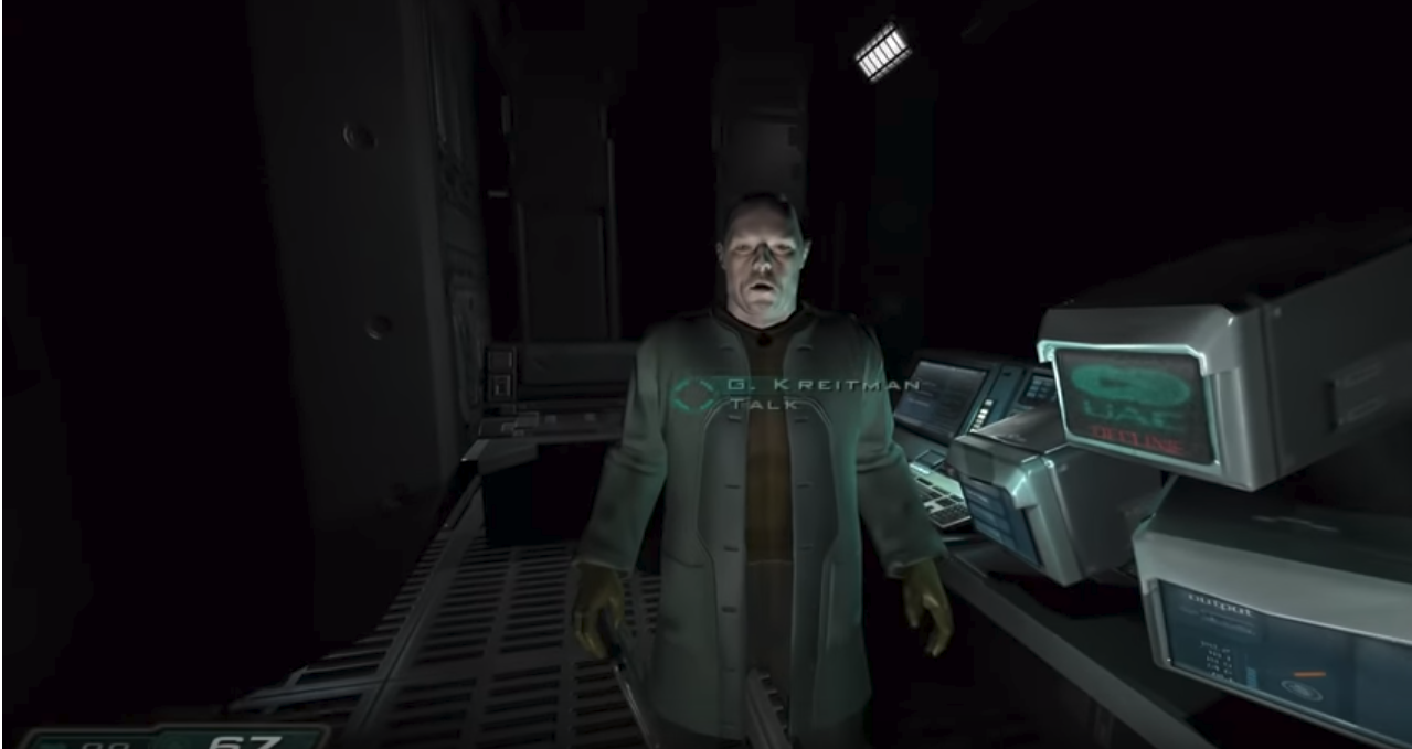
But when your graphics chips comes up, there’s suddenly a zombie walking on your screen. Which is awesome!
![Zombie]()
All of this just to make the point: there’s something magic about working on something that puts an image on the screen.
So when I started to reverse engineer the Pano Logic device, getting the VGA interface up and running was the first target. Luckily, it’s also far easier to get going than Ethernet and USB.
![Pano VGA]()
After my short RISC-V detour, instead of getting back to Ethernet, I wanted get a real application going, and since ray tracing has been grabbing a lot of headlines lately, I wondered if something could be done.
My first experience with ray tracing was sometime in the early nineties, when I was running PovRay on a 33MHz 486 in my college dorm. And when thinking about a subject for my thesis, hardware accelerated ray-triangle intersection was high on the list but ultimately rejected.
On that 486, you could see individual pixels being rendered one by one, far away from real time, but when you do things in hardware, you can pipeline and do things in parallel.
Compared to today’s high-end FPGAs, the Pano Logic has a fairly pedestrian Xilinx Spartan-3E, but the specs are actually pretty decent when compared to many of today’s hobby FPGA boards: 27k LUTs, quite a bit of RAM, and 36 18x18bit hardware multipliers.
Is that enough to do ray tracing? Let’s find out…
The HW Platform
Pano Logic was a Bay Area startup that wanted to get rid of PCs in large organizations by replacing them with tiny CPU-less thin clients that were connected to a central server. Think of them as VNC replacements. No CPU? No software upgrades! No virusses!
The thin clients had a wired Ethernet interface, a couple of USB ports, an audio port and a video port.
All this was glued together with an FPGA.
The company has been defunct since 2013 and the clients are not supported by anything. But they are amazing for hobby purposes and can be bought dirt cheap on eBay.
There are 2 versions: the first one has a VGA video interface, later versions have a DVI port.
The VGA version uses the Xilinx Spartan-3E 1600. The DVI version a very powerful Spartan-6 LX150.
Both are very easy to open up and reuse for other applications, but only the Spartan-3E FPGA is supported by the free Xilinx ISE software.
Consequently, only the Spartan-3E PCB has been almost completely reverse engineered by yours truly. The Spartan-6 version requires a very expensive (thousands of dollars per year) license.
If you want to recreate this project verbatim, make sure that you buy one on eBay that has a VGA port!
Racing the Beam - Graphics without a Frame Buffer
The traditional way of doing computer graphics looks like this:
- Render an image to frame buffer A which is large enough to store the value of all pixels on the screen.
- While the previous step is on-going, send the previously calculated image that’s stored in an alternate framebuffer B to the monitor.
- When you’re doing rendering your images, start sending the contents of frame buffer A to the monitor and render the next image in frame buffer B.
This setup has the huge advantage that you decouple render time and monitor refresh rate, and it’s used in all modern graphics system.
But there are a lot of pixels on a screen, and even for a 640x480 resolution and 24 bits-per-pixel, you need 7.3M bits per frame buffer, and you need two of those. So that’s 14.5Mbits of memory. The FPGA on the Pano Logic has only 648Kbit of block RAM.
The Pano box has 32MByte of DRAM on the board, more than enough. All the SDRAM IO connections to the FPGA have been mapped out, and Xilinx has an SDRAM memory controller generator, so using that should be a breeze, right?
Alas, no. The generator only supports regular DDR SDRAM. It does not support the LPDDR that’s used by the Pano. Designing a custom DRAM controller isn’t super hard, but it’s a major project in itself, one that I didn’t want to start just yet.
So using the SDRAM was out. And with that all traditional graphics rendering methods.
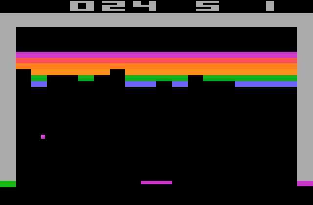
When you can’t use memory to store your image, you go back to a technique that was used more than 40 years ago in the Atari 2600 VCS: you race the beam! A CRT monitor paints an image by lighting up the phosphor on the screen with an electron beam from top to bottom and from left to right.
Back in those days, memory was extremely expensive, so to save on cost, they dropped the frame buffer and replaced it by a line buffer. It was up to the CPU to render the next line before the previous one was sent to the screen. If the CPU did not finish in time, the TIA video chip would just send the previous line again.
![Atari 2600 Breakout]()
(Picture (c) AtariAge)
We can take this technique to its ultimate conclusion where you not only replace the frame buffer by a line buffer, but where you drop the line buffer completely: if you are able to calculate each pixel on-the-fly exactly when the video output block wants it, you don’t need memory at all!
Now most graphics rendering techniques don’t build the image in pixel scan order: they’ll first paint the background, then they draw a triangle here and a triangle there, and eventually the whole image comes together.
But ray tracing is not like that: you shoot a ray from a virtual camera through a pixel to the scene and calculate the value of that pixel. Contempary ray tracing software choses the pixels in a stochastic order: essentially randomly distributed across the image. The benefit of this is that you see the whole image at once while it slowly refines into a high quality image. But that’s totally not necessary: you can just as well chose the pixels in scan order.
And if you’re able to calculate one pixel per pixel clock, you end up with a ray tracer that’s racing the beam!
One Pixel per Clock Ray Tracing
Ray tracing algorithms typically render scenes with a lot of triangles. The algorithm injects a ray into the scene, and figures out the closest intersecting triangle. If there are hundreds of thousands or more triangles, it uses hierarchical bounding box acceleration structures to reduce the number of ray/triangle intersections.
Once it has found the closest object, it calculates a base color and then casts a bunch of secondary rays into the scene to figure out light spots, shadows, reflections, refractions etc.
Doing all of that in a single clock cycle is a bit of a challenge, so there were some consequences and trade-offs.
First of all, if you have only 1 clock to calculate something, you are forced to calculate in parallel whatever you can, and if that’s not possible, you do it in a rigid pipeline: yes, it can potentially take many cycles to calculate one pixel, but you can issue the calculation of a new pixel each clock cycle, so you still end up with one pixel per clock at the output.
It also means that all the geometry of the scene is transformed into math operations that are embedded in the pipeline. Do you want one more sphere? Well, that will cost you all the hardware needed to calculate a ray/sphere intersection, the reflected ray, the sphere normal etc.
But wait, it gets worse! One of the main benefits of ray tracing are the ease by which it can render reflections. It’d be a shame if you couldn’t show that off. Unfortunately, reflection is recursive: if you have 2 reflecting objects, light rays can essentially bounce between them forever. You’d need an infinite amount of hardware to do that in one clock cycle… but even if you limit reflections to, say, 2 bounces, you’re still looking at a rapid expansion of math operations, and thus HW resources.
Or you chose the alternative: only allow 1 reflecting object in the scene. :-)
Since our FPGA is really quite small, there was a strict limit on what could be done. So the decision was made to have a scene with just 1 non-reflecting plane and 1 reflecting ball.
A Floating Point C Model
For a project with a lot of math, and a lot of pixels (and thus potentially very large simulation times), it’s essential to first implement a C model to validate the whole concept before laying things down in RTL.
First step is to simply use floating point. Converting to a format that’s more suitable for an FPGA is for later.
It didn’t take long to get the first useful pixels on the screen:
![cmodel1_plane]()
The code is almost trivial. I decided on pure C code without any outside libraries, so I had to create my own vector structs. I made a lot of changes to those along the way.
I used the scratchapixel.com ray-tracing tutorial code as the base for ray/plane and ray/sphereintersection.
A bit more code resulted in this:
![cmodel2_ray-sphere-intersection]()
and finally this:
![cmodel3-reflection.png]()
This was the point where it was time to check if this could actually be built: how many FPGA resources would it need make calculate this kind of image?
The code is still quite simple, but there are square roots, reciprocal scare roots, divisions, vector normalization, vector multiplications etc.
From Floating Point to Fixed Point
Ray tracing requires a lot of math operations with fractional numbers. The default to-go-to way to deal with fractional numbers on an FPGA is fixed point arithmetic. It’s essentially binary integer arithmetic, but the decimal… well… binary point is somewhere in the middle of the bit vector.
After each operation, it’s up to the user to make sure the binary point is adjusted: for an add/subract, no adjustements are needed, but for pretty much all other operations you need to shift the binary point back to get it back where it belongs: when you multiply 2 fixed point numbers with 8 fractional bits, the result will be one with 16 fractional bits. So you need to right shift by 8 to get back to 8 fractional bits.
This can all be automated with some specific rules, but some manual tuning may be needed due to resource restrictions.
For example: most FPGAs have 18x18 bit multipliers. If your 2 operands are 24-bit fractional numbers with 8 integer and 16 fractional bits, then you can stay within the 18 bit restriction by dropping the lower 6 fractional bits for both operands. The resulting 18x18 multiplication will have 16 integer and 20 fractional bits. After dropping 4 additional fractional bits and 8 MSBs, you’re back at a 24-bit fractional number.
In other words: 8.16 x 8.16 -> 8.10 x 8.10 = 16.20 -> 8.16
That’s something you can easily automate.
But what if operand A is a component of a normalized vector which is never larger than 1? And the operand B is always a rather large integer without many meaningful fractional bits?
In that case, it’s better to drop unused integer bits from the operand A and fraction bits from operand B.
Like this: 8.16 x 8.16 -> 1.17 x 8.10 = 9.27 -> 8.16
The end result is the same 8.16 fixed point format, but given the particular nature of the 2 operands, the second result will have a much better accuracy.
The disadvantage: it requires manual tuning.
In any case, the big take-away is this: fixed point works, but it can be a real pain. It’s great when most operands are all roughly within the same range (as is often the case for digital communications processing), but that’s not really true for ray tracing: there are numbers that will always be smaller or equal than 1, but there are also calculations with relatively large intermediate results.
Instead of writing a second, fixed point, C model, I did something better: I changed the code to calculate both floating and fixed point results for everything. This has the major benefit that the results of all math operations can be cross-checked against each other to see if they start to diverge in some big way.
A disadvantage is that all operations had to be converted into explicit function calls, even for basic C operations.
Here’s what the code looks like:
A scalar number:
typedef struct { float fp32; int fixed; } scalar_t;scalar_t add_scalar_scalar(scalar_t a, scalar_t b) { scalar_t r; r.fp32 = a.fp32 + b.fp32; r.fixed = a.fixed + b.fixed; ++scalar_add_cntr; check_divergent(r); return r; }Notice the
check_divergentfunction call. That’s the one that checks if the fp32 and fixed point numbers are still more or less equal.scalar_t _mul_scalar_scalar(scalar_t a, scalar_t b, int shift_a, int shift_b, int shift_c) { scalar_t r; r.fp32 = a.fp32 * b.fp32; r.fixed = ((a.fixed>>shift_a) * (b.fixed>>shift_b)) >> shift_c; ++scalar_mul_cntr; check_divergent(r); return r; }Here you can see how I allow for flexibility in chosing pre- and post-operation shift parameters to get the best precision and result.
In this version of the code, I’m taking a few liberties with the square root operation, but here’s the generated image:
![fixed_point.png]()
It doesn’t look half bad! The only real issue are the jaggies around the boundary of the sphere. Let’s ignore those for now. :-)
Math Resource Usage Statistics
Remember how we need to be able to fit all math operations in the FPGA in parallel? Now is the time to see how much is really needed.
If you paid any attention, you probably noticed the
++scalar_add_cntr;operation in the scalar addition code snippet above. That line is one of the usage counters that keep track of all types of scalar operations that are performed to calculate a single pixel.Here are all the operations that are being tracked:
int scalar_add_cntr         = 0;
int scalar_mul_cntr         = 0;
int scalar_div_cntr         = 0;
int scalar_sqrt_cntr        = 0;
int scalar_recip_sqrt_cntr  = 0;
When setting right
#definevariable, you end up with the following result:scalar_add_cntr: 46 scalar_mul_cntr: 48 scalar_div_cntr: 2 scalar_sqrt_cntr: 1 scalar_recip_sqrt_cntr: 2
That biggest issue here are the number of multiplications: 48 is quite a bit larger than the 36 HW multipliers of our FPGA.
The additions shouldn’t be a problem at all. Hardware division is notoriously resource intensive and unexplored territory, but square root should be doable with some local memory lookup. Which is fine: since we’re racing the beam, we don’t need to use the local RAMs for anything else anyway.
Scene Math Optimization
Here’s one interesting observation: a lot of the math in the current scene is not really necessary.
ray_t camera = {
    .origin   = { .s={ {0,0}, {10,0}, {-10,0} } }
};

plane_t plane = {
    .origin = { .s={ {0, 0}, {0, 0}, {0, 0} } },
    .normal = { .s={ {0, 0}, {1, 0}, {0, 0} } }
};

sphere_t sphere = {
    .center = { .s={ {3, 0}, {10, 0}, {10, 0} } },
    .radius = { 3 }
};
There are a lot of numbers here that can be made constant. If we keep the plane in the same place and horizontal at all times, that’s a lot of zeros and fixed numbers and math that can be optimized away.
When you search in the code for
SCENE_OPT, you’ll find a bunch of these kind of optimizations.There’s a good example of this in the plane intersection function:
#ifdef SCENE_OPT
    // Assume plane is always pointing upwards and normalized to 1.
    denom = r.direction.s[1];
#else
    denom = dot_product(p.normal, r.direction);
#endif
That’s a vector dot product (3 multiplications and 2 additions) reduced to just 1 assignment!
These are the usage stats after the dust settles:
scalar_add_cntr:        32
scalar_mul_cntr:        36
scalar_div_cntr:        2
scalar_sqrt_cntr:       1
scalar_recip_sqrt_cntr: 2
This isn’t too bad! There are 36 HW multipliers in the FPGA, so that’s an exact match.
Start Your SpinalHDL RTL Coding Engines! Or… ?
With all the preliminary work completed, it was time to start with the RTL coding.
After the excellent experience with my MR1 RISC-V CPU, SpinalHDL is now my hobby RTL language of choice. It even has a fixed point library!
First step is to get an LED blinking.
And then the coding starts.
Or that was the initial plan.
But for some reason, I just didn’t feel like implementing this whole thing using fixed point. After all, someone else had already created this whole library. Where’s the fun in that?
What happened was one of the best parts of doing something as a hobby: you can do whatever you want. You can rabbit-hole into details that don’t matter but are just interesting.
I got interested into limited precision floating point arithmetic. I adjusted the C model to support
fpxx, a third numerical representation in addition to fp32 and fixed point.typedef fpxx<14,6> floatrt; typedef struct { float fp32; floatrt fpxx; int fixed; } scalar_t;And then I spent about a month researching and implementing floating point operations as its own C model and RTL.
The resulting Fpxx library is a story on itself.
Conversion to 20-bit Floating Point Numbers
Since the fpxx library was implemented using C++ templates, it was trivial to update the ray tracing C model to use it.
After some experimentation, the conclusion was that I could still render images with more or less the same quality by using a 13 bit mantissa and a 6 bit exponent. Reducing either one by 1 bit results in serious image corruption. Add 1 sign bit, and we have a 20-bit vector for all our numbers.
The fixed point implementation was using 16 integer, and 16 fractional bits and required making choices when doing multiplications. By moving to a 13-bit mantissa only a 14x14 bit multiplier is needed, and we don’t need to drop any bits when using the 18x18 bit HW multipliers. So that’s good!
Building the Pipeline
The time had finally come to build the whole pipeline.
To make the conversion even easier, some C model code was updated with additional intermediate variables to get a close match between the C model variable names and RTL signals.
Here’s a good example of that:
Old:
    scalar_t c0r0_c0r0 = dot_product(c0r0, c0r0);
    d2 = subtract_scalar_scalar(d2, mul_scalar_scalar(tca, tca));
New:
    scalar_t c0r0_c0r0 = dot_product(c0r0, c0r0);
    scalar_t tca_tca = mul_scalar_scalar(tca, tca);
    scalar_t d2 = subtract_scalar_scalar(c0r0_c0r0, tca_tca);
And the corresponding RTL code:
    //============================================================
    // c0r0_c0r0
    //============================================================
    val c0r0_c0r0_vld = Bool
    val c0r0_c0r0     = Fpxx(c.fpxxConfig)
    val u_dot_c0r0_c0r0 = new DotProduct(c)
    u_dot_c0r0_c0r0.io.op_vld     <> c0r0_vld
    u_dot_c0r0_c0r0.io.op_a       <> c0r0
    u_dot_c0r0_c0r0.io.op_b       <> c0r0

    u_dot_c0r0_c0r0.io.result_vld <> c0r0_c0r0_vld
    u_dot_c0r0_c0r0.io.result     <> c0r0_c0r0

    //============================================================
    // tca_tca
    //============================================================
    val tca_tca_vld = Bool
    val tca_tca     = Fpxx(c.fpxxConfig)

    val u_tca_tca = new FpxxMul(c.fpxxConfig, pipeStages = 5)
    u_tca_tca.io.op_vld <> tca_vld
    u_tca_tca.io.op_a   <> tca
    u_tca_tca.io.op_b   <> tca

    u_tca_tca.io.result_vld <> tca_tca_vld
    u_tca_tca.io.result     <> tca_tca

    //============================================================
    // d2
    //============================================================
    ...
SpinalHDL LatencyAnalysis Life Saver - Automatic Latency Matching
This section was spun off into its own blog post.
Progression to C Model Match
Implementing a ray tracing pipeline for the first time requires quite a bit of RTL without any kind of feedback: you need a lot of pieces in place before you can finally render an image.
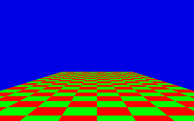
In my case, I decided to implement all the geometry before attempting to get an image going on the monitor.
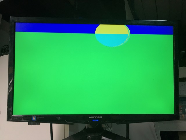
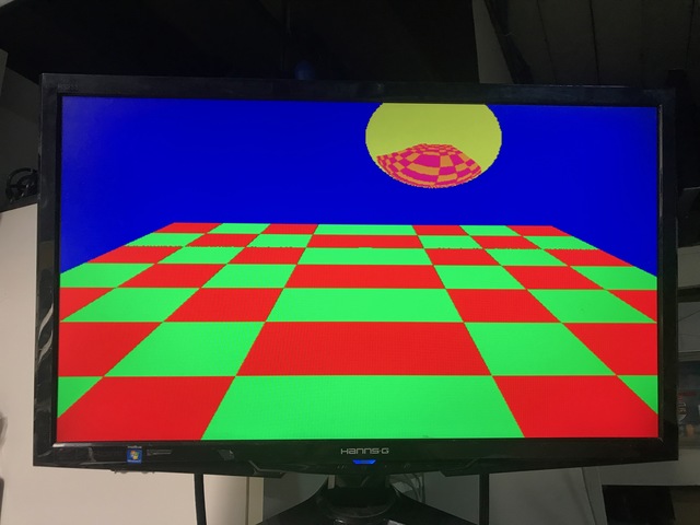
I hadn’t implemented the plane checker board colors yet, so I expected 4 different colors: the sky (blue), the plane (green), a sphere reflecting the sky (yellow), and a sphere reflecting the plane (cyan.)
Once everything compiled without syntax and pedantic elaboration errors (another huge benefit of SpinalHDL), I was ready to fire up the monitor for the first time, and was greeted with this:
![Progression 1]()
Not bad huh?!
I had flipped around the Y axis, so you only so that top of the sphere.
Plane intersection always passed because I had forgotten to clamp the intersection point to only be in front of the camera.
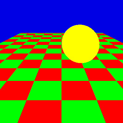
But, hey, something that resembles a circle! Let’s fix the bugs…
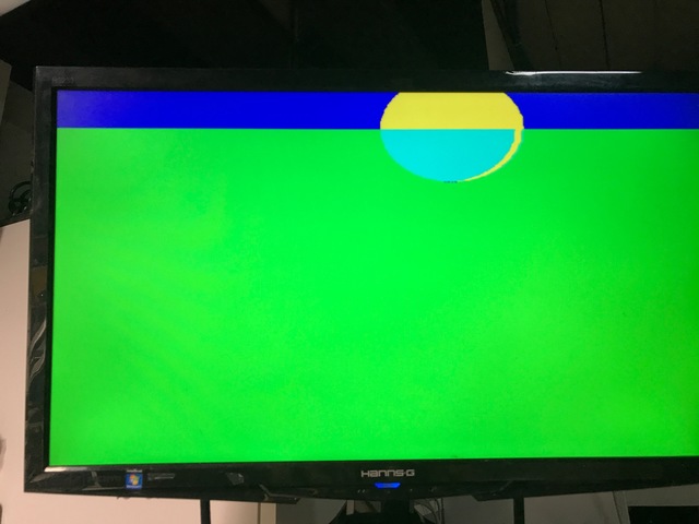
![Progression 2]()
Much better!
Those weird boundaries on the right of the sphere? Those were a pipeline bug in my FpxxAdd block that only showed up when using less than 5 pipeline stages (which was my only testbench configuration.)
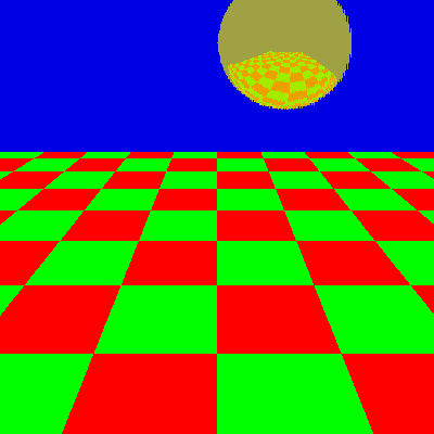
![Progression 3]()
Another pipelining bug…
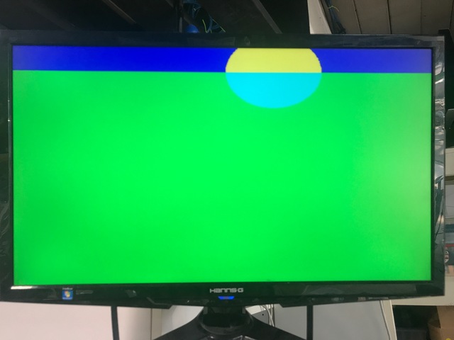
![Progression 4]()
Excellent! It’s just a coincidence that the plane (green) and the reflected plane (cyan) align horizontally: that’s because the camera is concidentally at the same level as the center of the sphere, and the plane is running all the way to infinity.
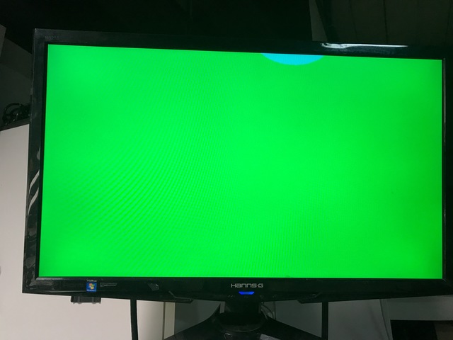
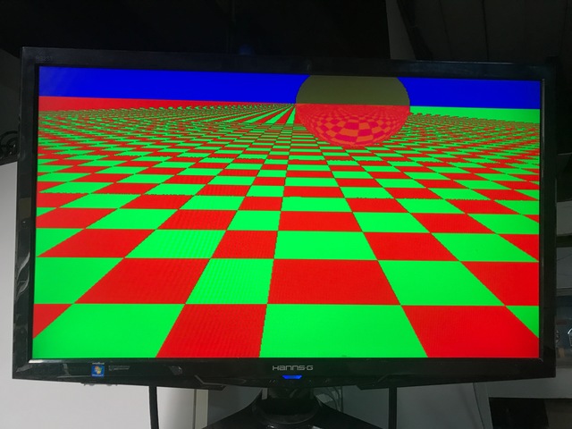
![Progression 5]()
Checker board is ON!
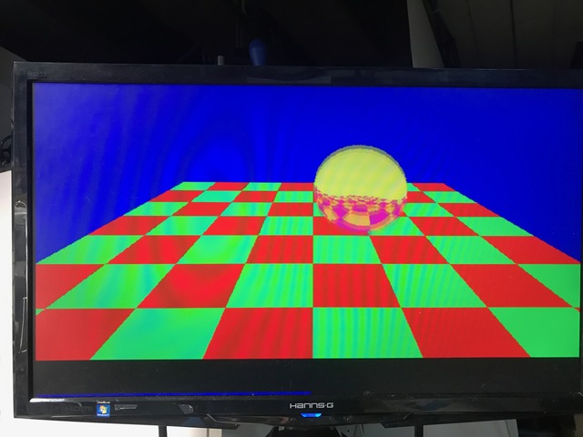
![Progression 6]()
Static Render is a GO!
![Progression 7]()
See the fuzzy outlines around that sphere?
That’s because I took the picture while it was moving!
https://player.vimeo.com/video/302770385
Intermediate FPGA Synthesis Stats - A Pleasant Surprise!
At this point, the RTL has progressed past the point where the C model development was stopped: the sphere is bouncing, which reduces the amount of math that can be optimized away since the sphere Y coordinate is now variable.
Yet we were able to fit this into the FPGA? Let’s look at the actual FPGA resource usage:
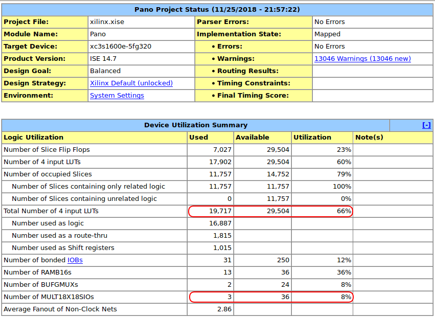
![Xilinx ISE Intermediate Stats]()
GASP!
We are only using 66% of the FPGA core logic resources despite the fact that we’re also using only 3 out of 36 HW multipliers!
It turns out that the creaky old Xilinx ISE synthesis and mapping functions don’t infer HW multipliers when their inputs are only 14x14 bits.
This opens up the possibility for more functionality!
The logic synthesizes at 61MHz. Plenty for a design that only needs to run at 25MHz which is the pixel clock for 640x480@60Hz video timings.
A Sphere Casting a Shadow and a Directional Light
A bouncing sphere is nice and all, it just didn’t feel real: there is no sense of it approaching the plane before it bounces, and the sphere surface is just too flat.
It needs a directional light that shines on the sphere and casts a shadow.
That’s trival to implement: we already have a
sphere_intersectblock! All we need to do is add a second instance, shoot a ray from the ray/plane intersection point to the light at infinity, and check if it intersects the sphere along the way.Similarly, already have the reflection vector of the eye-ray with the sphere. If we do a dot product with that vector with light direction vector and square it a few time, we get a very nice light spot on the sphere.
This was quickly added to the C model, and almost just as quickly to the RTL:
Much better!
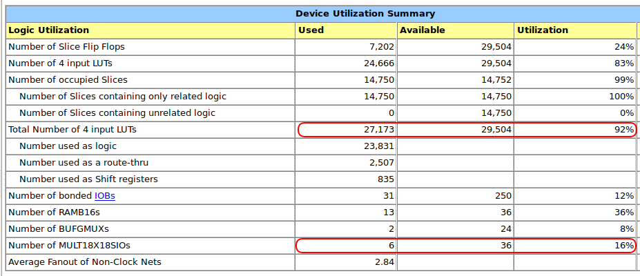
Notice how the shadow on the plane is also visible on the sphere. This is what makes ray tracing such an appealing rendering technique!
The additional features bumped the core logic stats up from a comfortable 66% to a much tighter 92%. The number of HW multipliers doubled as well.
![Xilinx ISE Shadow and Light Stats]()
SpinalHDL - Selectively Using HW Multipliers
It’s usually pretty simply to add hints to the synthesis tool about how to implement certain HW blocks, and I expected the same for forcing Xilinx ISE to use HW multipliers.
But one way or the other, I wasn’t able to get that to work.
The brute-force alternative is to hand-instantiate the FPGA-specific multiplier primitives, so that’s what I did instead.
It requires just a tiny bit of work in SpinalHDL:
- First you define a black box of the primitive that you want to add.
- And then you simply treat that black box as any other component.
Since I want to be able to mix HW and ‘soft’ multipliers, built from regular logic elements, I added the option for each FpxxMul component to use one or the other.
One issue is that absense of a Verilog simulation model for the HW multiplier. Writing one myself would have been the best option, but I decided to have one global variable that allows me to disable all HW multipliers.
When running simulation, I disable them. When creating a synthesis netlist, I enable them.
It works like this:
- For each Fpxx building block, I have a configuration class. For example, for FpxxMul, there is FpxxMulConfig.
case class FpxxMulConfig(
    pipeStages      : Int     = 1,
    hwMul           : Boolean = false
    ){
}
I then have some global instances of this configuration class. One with HW multiplier enabled, and one without.
And, finally, hwMulGlobal is the global selector that decides between using HW multipliers or not.
object Constants {
    val hwMulGlobal = true
    ...
    def fpxxMulConfig   = FpxxMulConfig(pipeStages = 5)
    def fpxxHwMulConfig = FpxxMulConfig(pipeStages = 1, hwMul = hwMulGlobal)
    ...
    def dotHwMulConfig      = DotProductConfig(hwMul = hwMulGlobal)
    def rotateHwMulConfig   = RotateConfig(hwMul = hwMulGlobal)
}
After adding the 2 rotation matrix operations (see below), logic element usage was at 99%. After enabling HW multipliers, I went down to around 80% or so!
Camera Movement and Flexibility - Bringing in a CPU
Everything up to this point was implemented completely in hardware. The camera had a fixed location, and the its orientation was static as well.
Ideally, you’d like to be able to move the camera around and point in any direction, left and right, and up and down.
That requires 2 rotations that must be performed for each ray. It requires sine and cosine of the rotation angles. It also requires something that updates the position and angles once per frame.
It’s basically something you’d do on with a CPU!
Adding the rotation was once again trivial. First added to the C model, then in hardware.
And since my previous project was a small RISC-V project, integrating that was very easy as well.
Once the CPU was in place, I could remove the hardware that calculated the bouncing ball (gaining some logic elements in the process), but now the sphere position, the camera position and the rotations were fully programmable. Which removed the ability of the synthesis tool to optimize logic out.
The CPU runs a small program, once per frame, that updates the position of the camera, looks up sine and cosines from a lookup table etc. It doesn’t a particularly interesting thing with the camera, but it’s good enough for a technology demo.
Text Overlay - The Final Step
I wanted to show some text on the screen. I already had a Verilog VGA text generator, so I converted that one to SpinalHDL and called it a day.
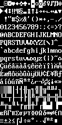
I chose the old IBM PC font for this.
Some characters, like the ‘m’ and the ‘w’ touch the characters on the left and right in some cases. That’s a bit ugly, so I decided to use a 9 pixel width instead of the standard 8 pixels. But now the spacing between other characters is a little bit off…
![IBM PC VGA Font]()
Final Toplevel Pipeline
This is the complete toplevel pipeline:
![Toplevel Pipeline]()
Along the top, you see the steps that are needed to generate the primary rays that are shot from the viewer into the scene.
Then from the top to bottom are all the steps to calculate the final pixel.
One thing that wasn’t mentioned before is the fact that there’s only 1 ray/plane intersection block: if you first do the sphere intersection, you can use the result of that operation to decide whether you want to calculate the intersection of the primary ray with the plane (when the ray does not intersect the sphere) or the intersection of the secondary, sphere reflected ray with the plane (when the ray does intersect with the sphere.) That saves quite a bit of hardware!
There are the ray/sphere intersection and ray/plane intersection blocks:
Sphere:
![Sphere Intersection Pipeline]()
Plane:
![Plane Intersection Pipeline]()
And when flatten all these blocks, you get this floating point monster pipeline:
![Exploded Top View]()
Use your browser’s zoom function to zoom in on the individual operations!
Total Resource Usage and Critical Path
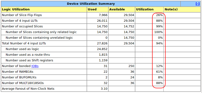
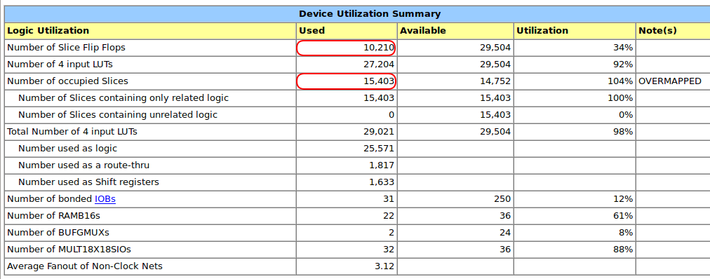
Here’s the final FPGA resource usage:
![Xilinx ISE]()
94% of all LUTs is seriously disappointing: I should have pushed harder to get that closer to 99% by adding some additional features, but I was ready to move on to some new project.
One feature that’s relatively easy to implement would be to render a textured bitmap on top of the plane.
There are still 4 multipliers left as well.
RAM usage is split between CPU RAM, and a special table for the FpxxDiv, and lookup tables for the FpxxSqrt and the FpxxRSqrt.
A quick look at the FPGA floorplan confirms that it’s packed pretty tightly:
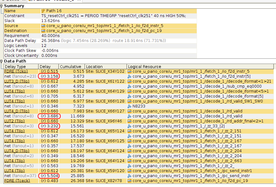
![Worst Case Path 1]()
The stuff in white is the critical path. Surprisingly enough, it’s somewhere in the MR1 CPU, but it’s still passing by a mile: target frequency 25MHz, achieved frequency some 38MHz.
![Worst Case Path 3]()
The red circled items above show how the Xilinx ISE placer has made decisions with large routing delays. But there’s nothing wrong with that: timing is met after all…
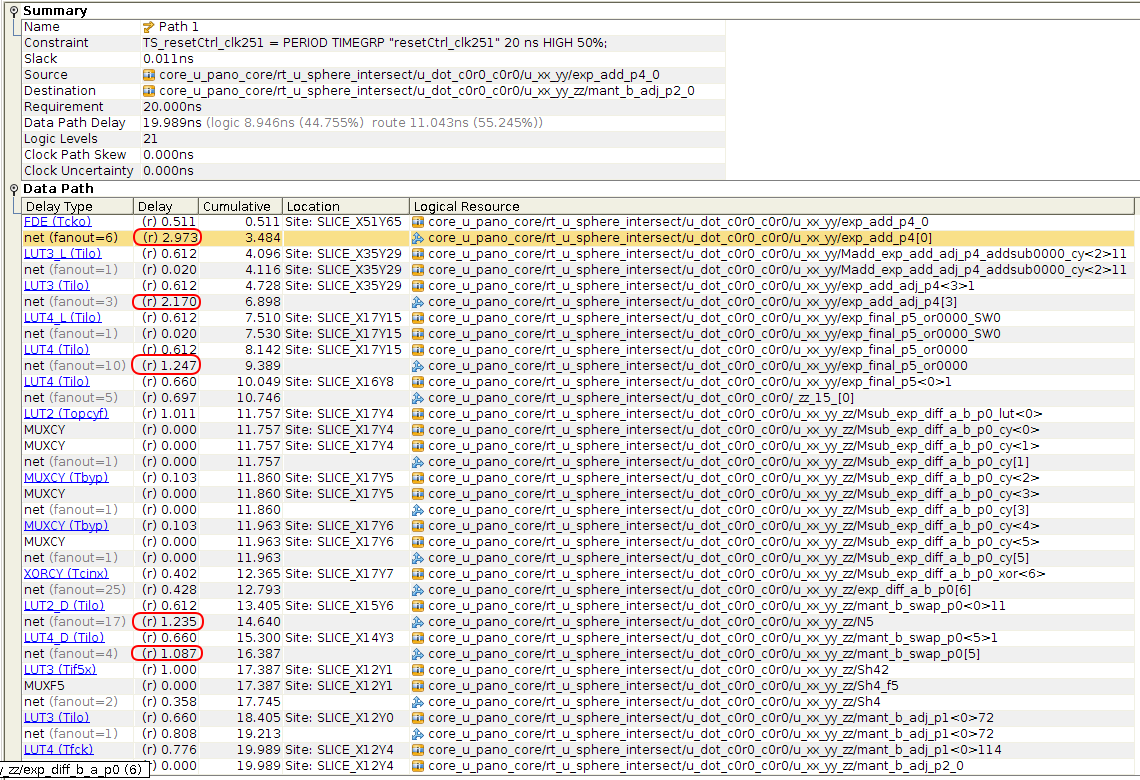
I wanted to see if I’d get better placement (and timing) results if I tightened the clock speed from 25MHz to 50MHz.
![Worst Case Path 4]()
It’s a bit harder to see, but timing is still met, and the critical path has moved from the CPU to half floating point multiplier and half floating point adder. Placement is a lot better, with only 2 routing delays that exceed 2ns and only 5 that exceed 1ns. We’re probably close to the limit if we don’t increase the amount of pipeline stages.
And, indeed, with the clock increased to 66MHz, I got a result that was worse than the previous one: only 45MHz instead of 50MHz. That’s not unusual: there’s always a random factor at play with this kind of algorithms.
I increased the number of pipeline stages in the floating point adders from 2 to 3. This increases the total pipeline depth from 82 <> to 105 and the number of flip-flops from 7966 to 10210.
Sadly, that’s too much of our little FPGA:
![FpxxAdd 3 Stages]()
The End
Ray tracing, floating point arithmetic, giving my RISC-V something useful to do, more SpinalHDL learning and pushing the Pano Logic Spartan-3E to its limits.
The end result is pretty much useless: there is no practical application where this kind of ray tracing would make sense. As soon as you add more (reflective) geometry to the scene, the amount of logic explodes.
But it was a lot of fun!
Here’s the end result again:
https://player.vimeo.com/video/303938705
References
-
Audio Playback, USB and Ethernet Connections
07/10/2018 at 06:17 • 0 commentsAfter a vacation and lots of World Cup quality time (Go Belgium!), the pace on the Pano Logic project has been picking up again.
Audio Playback
Audio playback was always high on the list and there’s a lot of progress on this front: I can play a 1KHz test tone when plugging in my headphones!
For reasons unknown, the speaker does not work, even after a long evening of trying as many settings as possible.
Still, with this milestone, I’m one step closer to using the Pano Logic box as a mini game console.
USB
The interface between the NXP ISP1760 and the FPGA has been completely mapped… I think. The chip has a 16-bit and a 32-bit mode. On this board, the 16-bit mode is used. I expect that it will be quite a bit of effort to get USB going. First step will simply to be get the FPGA to read and write registers and then we’ll see where it leads us.
Even though the ISP1760 has a built-in 3-way hub, there is an external SMSC USB2513 hub. I was told that the ISP1760 has some bugs in the hub, so that probably explains the presence of this SMSC chip.
The SMSC chip has an I2C interface, but was only able to identify a reset and a clkin signal between the FPGA and the SMSC chip. It’s possible that the default configuration is sufficient and that no further configuration is necessary.
Ethernet
A bunch of connections between the Micrel KSZ8721BL Ethernet PHY and the FPGA were identified as well. However, there are some signals that seem to be suspiciously not connected (e.g.
eth_txcandeth_pd_).Getting Ethernet to work would be incredibly nice, but it’s a pretty complex undertaking and lowest priority.
Next Up
I may spend a bit more time on getting the speaker to work, but the true challenge ahead will be USB: the Pano Logic box is almost useless if you can’t connect a keyboard to it.
(Originally published here.)
-
VGA is Up - VexRiscV CPU - Text Mode
06/04/2018 at 07:07 • 0 commentsPCB Reverse Engineering Progress
The most important resource are the connections between the FPGA and its surroundings. That information is captured in the top.ucf file.
Right now, I have the following interface have been completed:
- IDT ICS307 clock generator
This interface is not only complete, but there is also RTL that successfully programs the generator into creating the pixel clock for 1080p VGA video timings. The RTL can be found here.
- TI THS8135 10-BIT 240-MSPS VIDEO DAC
Nothing is more fun that having your own design generate and image and send it to a monitor, so this one had full priority. With this interface figured out, we can create the RGB signals. But that’s not enough! We also need:
- Connector between board and daughter board
VGA doesn’t have HSYNC and VSYNC embedded in the RGB signals: it has separate pins for that. In order to create video, I had to figure out how the FPGA controls HSYNC and VSYNC.
In the process, a lot of other signals were also identified: USB signals, VGA DDC I2C pins, button, and LED control. No project is officially alive without a blinking LED.
- Wolfson WM8750BL
Audio bringup soon!
- DDR2 SDRAM
VGA Bringup
With everything in place to create video signals, and some pretty simply RTL code, you can now see the following:
Under the Hood: VexRiscV CPU
With video figured out, it’s time to move to bring up other interfaces. Audio is quite simple, so that’s high on the list.
But we really need a CPU to make that kind of bringup easy. For example, the Wolfson CODEC is configured through I2C. I’m already using a bit-banged I2C master on a Nios2 for my eeColor Color3 project. I want to do the same here.
That’s why the project now also has a VexRiscV!
A seperate post will go into the details about the specifics of this RISC-V core, but the most important reasons to choose this one over the ubiquitous PicoRV32 are:
- Xilinx ISE 14.7 and PicoRV32 aren’t friendly.
It’s totally possible to make it work with relatively minor RTL edits, but that was only true when you don’t use using the HW multiplier. Using the multiplier breaks the terrible Xilinx software. Meanwhile, ISE was able to grok the VexRiscV on first try, multiplier and all.
- The VexRiscV is much faster.
Or better, the PicoRV32 is really slow, coming in at 3 to 7 cycles per instruction. The VexRiscV is just as configurable as the PicoRV32 and can go at one cycle per instruction without trying very hard. (It’s currently running at 2 cycles per instruction though.)
It’s not that we need a faster CPU for our current purposes, but the amount of logic resources for the VexRiscV is almost the same as for the PicoRV32. And it’s fun to explore different cores. So why not?
At this time, the CPU is only used to blink the LEDs (yay!). That’s because some other infrastructure is necessary to really start using it: as way to tell the user what’s going on. That’s why the following was developed:
Text Mode Output
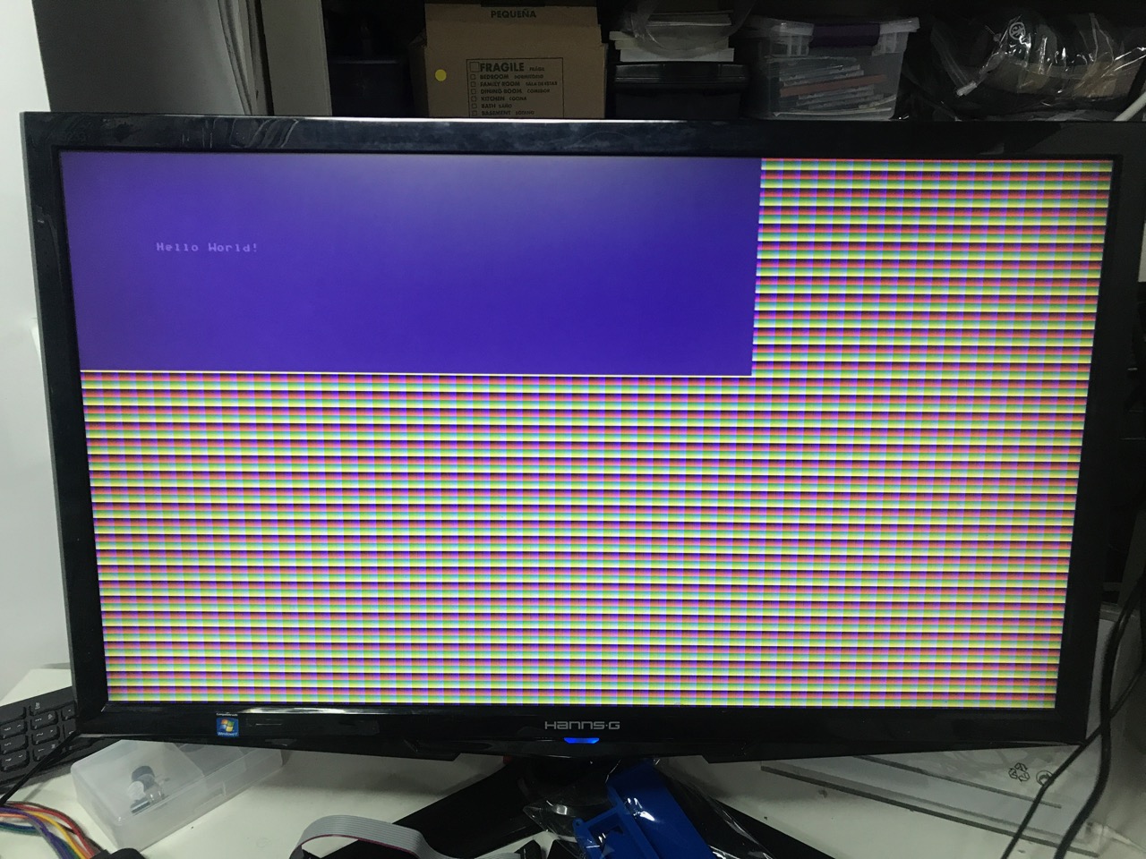
And as of today, there is also a character generator:
![Hello World!]()
The GitHub repo is always in a state of flux, but that example can be generated by syncing to this commit.
The screen buffer hasn’t been connected to the CPU yet, but once that’s done, everything will be in place to start driving other parts of the PCB.
(Sadly, the Commodore 64 font will be replaced by the vintage IBM 8x12 character set, since the latter is ASCII mapped out of the box.)
Conclusion
Lots of progress. More to come!
Next step: getting audio-out to work.
- IDT ICS307 clock generator
-
Works have Started
05/11/2018 at 06:27 • 0 comments(Also published here.)
After transcribing the data from previous reverse engineering efforts , and an insane amount of effort to Xilinx ISE 14.7 to work with my Digilent JTAG clone, I've started for real with the mapping out the pins of the FPGA.
The PCB is remarkable in that all the balls of the FPGA and the SDRAM BGAs have an accessible via.
That makes it really easy to figure out all the connections between them. So that's the work that got completed first.
The remainder of the chips are some form of a QFP. You can figure out the connections either by installing a ChipScope (similar to how I did some of the eeColor Color3 pins), but that doesn't work inputs to the FPGA.
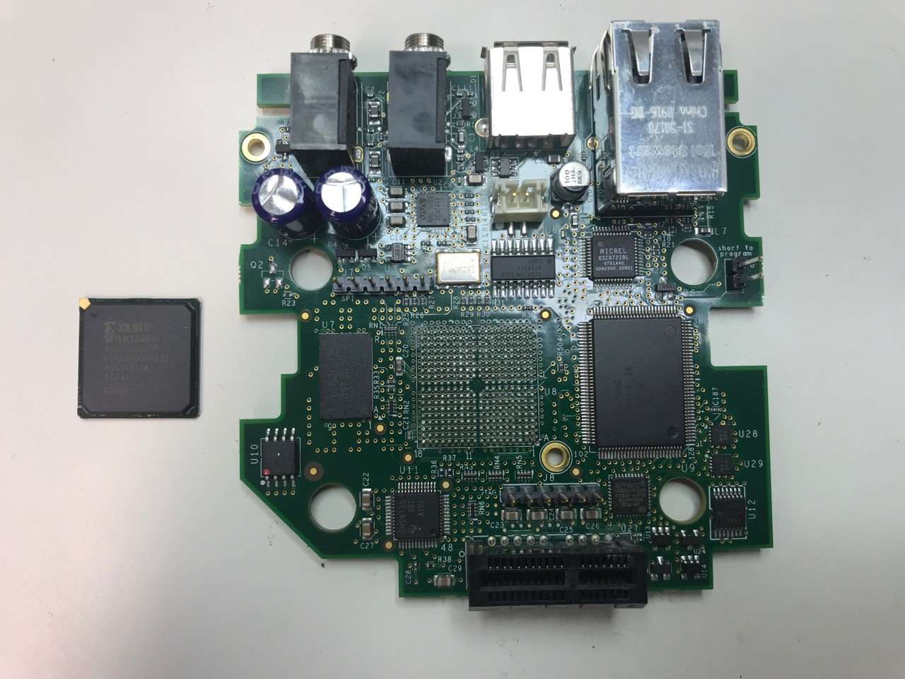
It'd be much easier to remove the FPGA from the board and Ohm things out that way.
But that'd be a deliberate act of violence and destroy the board.
Well... I bought a lot of 5 of them for $45.
![]()
So off when the FPGA. Feel dirty, man.
I've now mapped out the full connection between the FPGA and the TI VGA Out chip. At this point, this should enable me to send an image to a monitor, but VGA is so old now that I couldn't find a VGA cable at home (or even at work.)
While waiting for a cable, I've started mapping out the USB host chip as well.
-
Acquisition of the Goods!
04/14/2018 at 20:39 • 0 comments(Also published here.)
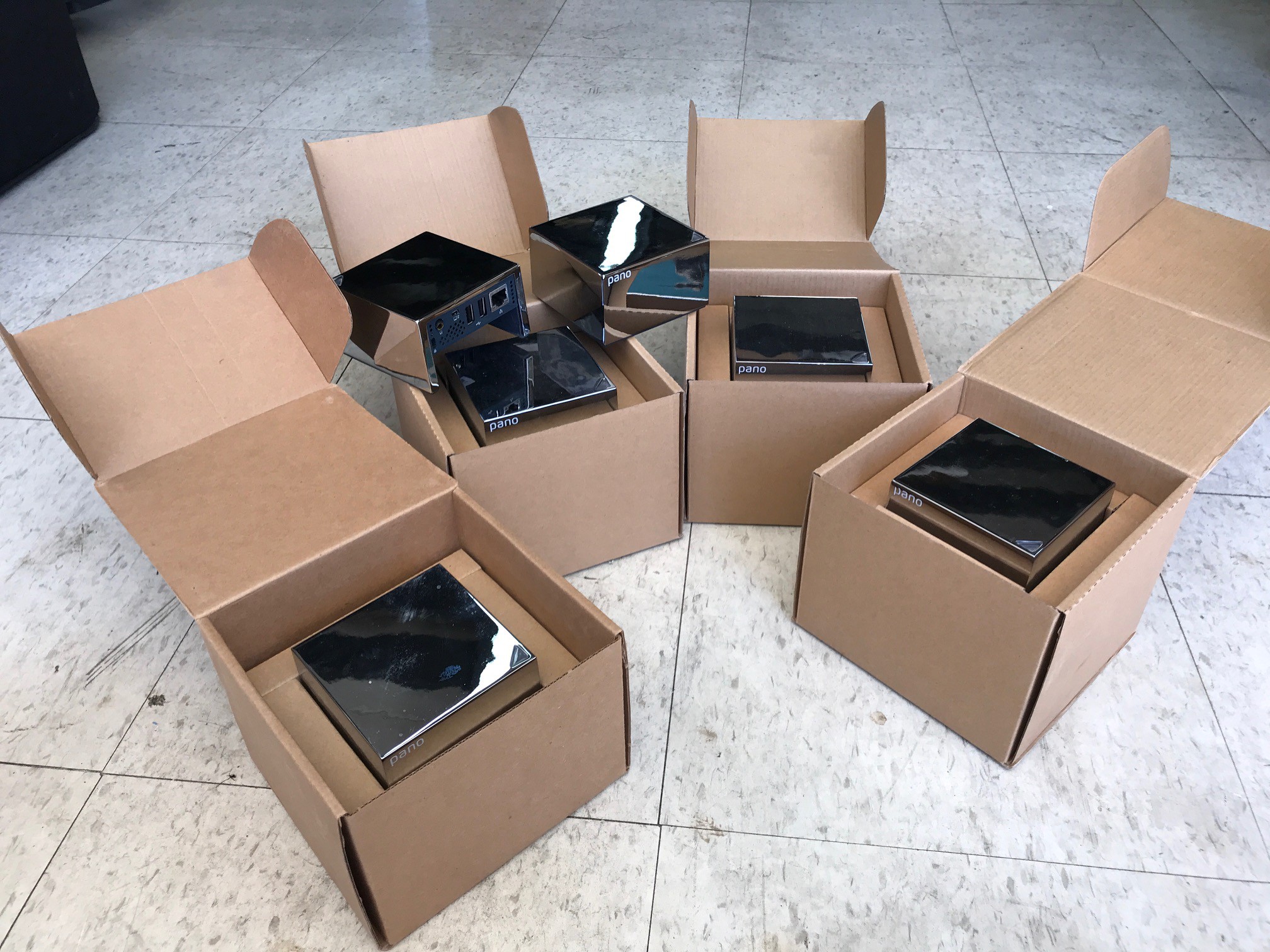
The first step has been completed: acquisition of the goods!
I mistakenly first bought a gen 2 for $10, which can't be used due to lack for free Spartan 6 license.
But today, a lot of 5 gen 1s arrived which were purchased for a whopping $45 on eBay. Here's the full family!
![]()
$9 per device is not bad, but I could have done better: there was another offer on eBay of 33 devices for the low low price of $150, though 9 of those were gen 2. Still 24 useable unit would be only $6 each.
But 5 should be sufficient to break a few and still have enough left for real projects.
The real work will have to wait until I get bored with the Color 3 work.
Pano Logic Zero Client G1
Documenting the internals of the first gen for hobby use