Intro: High-Precision Temperature Controller

-------------------------------------------------------------------------------

The NTCs (negative temperature coefficient) are special thermistors which change the resistance depending on the temperature. Those NTCs combined with the with calibration method discovered by Stanely Hart and John Steinhart as described in the article "Deep-Sea Research 1968 vol.15, pp 497-503 Pergamon Press" is the best solution in my case. The paper discusses methods of wide range temperature measurements (hundreds of Kelvins...) with those type of devices. In my understanding, coming from an engineering background, the simpler the system/sensor the better. No one wants to have something super complicated under the water, on kilometer depths which can cause issues while measuring temperature there only due to their complexity. I doubt the existence of the sensor to function similarly, maybe thermocouple will, but it requires some support circuitry and it is for extreme precision cases. So let's make the use of those two, for the cooling system design which has several challenges. Some of them are: noise level, the effective sampling of the real-time value and possibly, all above mentioned in a simple and handy package for ease of repair and maintenance also, the costs per unit. Meanwhile writing the firmware, the setup got more and more tweaked and improved. At some point, I realized that it might as well become a standalone instrument due to its complexity.

Temperature Calibration by Steinhart-Hart

---------------------------------------------------------------------------

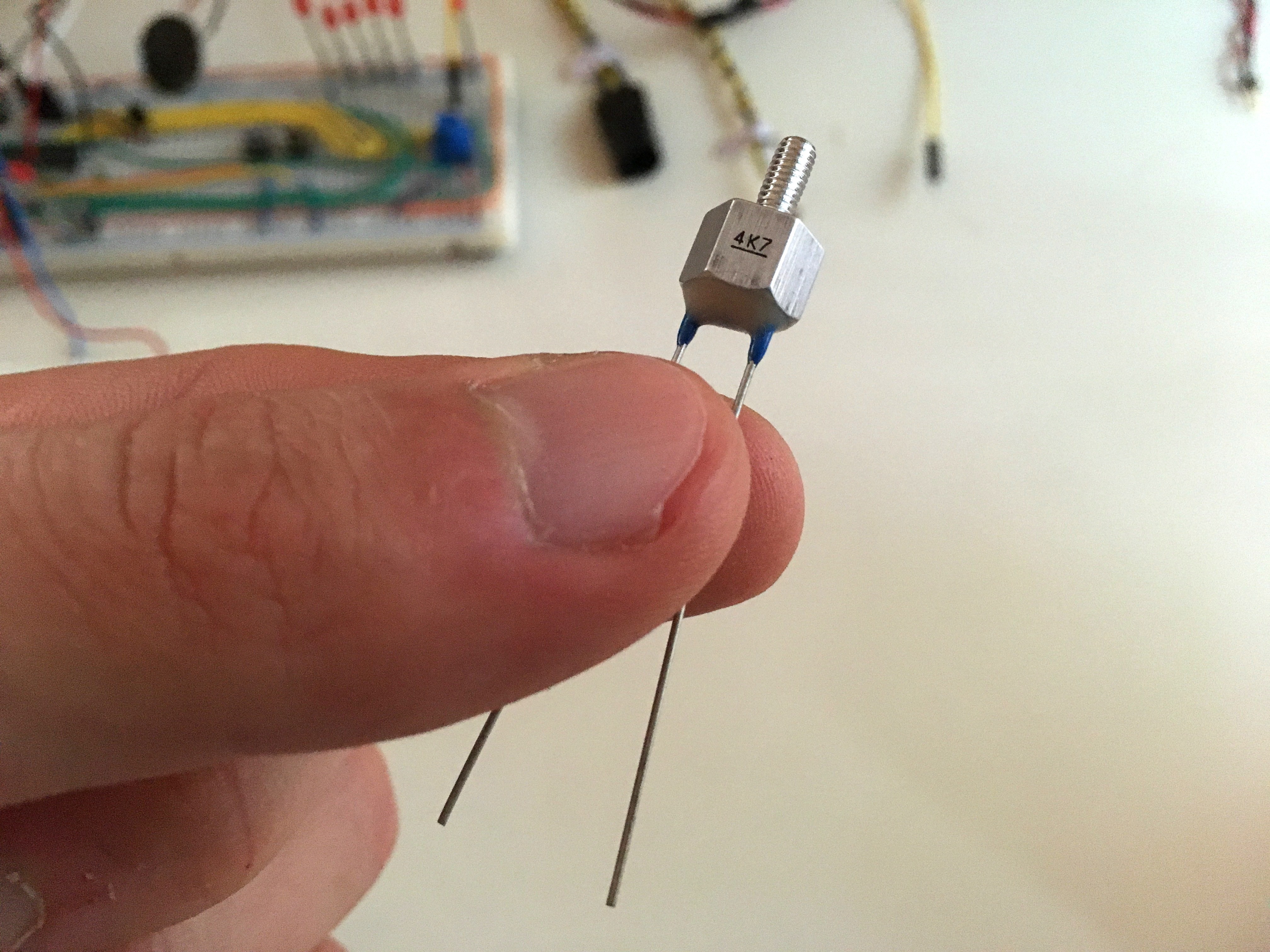
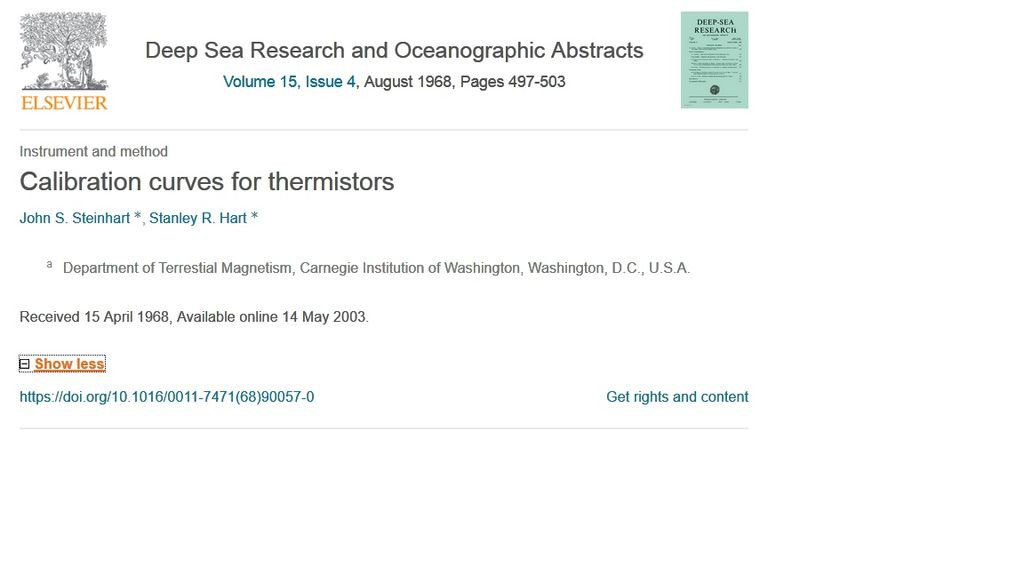
There is nice article in Wikipedia which will help to calculate the thermistor coefficients depending on needed temperature and thermistor range. In most cases the coefficients are super small and could be neglected in equation in its simplified form.

The Steinhart–Hart equation is a model of the resistance of a semiconductor at different temperatures. The equation is:

1 T = A + B ln ⁡ ( R ) + C [ ln ⁡ ( R ) ] 3 {\display style {1 \over T}=A+B\ln(R)+C[\ln(R)]^{3}}

where:

T {\display style T} is the temperature (in Kelvin) R {\display style R} is the resistance at T (in ohms) A {\display style A} , B {\display style B} , and C {\display style C} are the Steinhart–Hart coefficients which vary depending on the type and model of thermistor and the temperature range of interest. (The most general form of the applied equation contains a [ ln ⁡ ( R ) ] 2 {\display style [\ln(R)]^{2}}

term, but this is frequently neglected because it is typically much smaller than the other coefficients, and is therefore not shown above.)

Developers of the equation:

The equation is named after John S. Steinhart and Stanley R. Hart who first published the relationship in 1968.[1] Professor Steinhart (1929–2003), a fellow of the American Geophysical Union and of the American Association for the Advancement of Science, was a member of the faculty of University of Wisconsin–Madison from 1969 to 1991.[2] Dr. Hart, a Senior Scientist at Woods Hole Oceanographic Institution since 1989 and fellow of the Geological Society of America, the American Geophysical Union, the Geochemical Society and the European Association of Geochemistry,[3] was associated with Professor Steinhart at the Carnegie Institution of Washington when the equation was developed.

References:

John S. Steinhart, Stanley R. Hart, Calibration curves for thermistors, Deep-Sea Research and Oceanographic Abstracts, Volume 15, Issue 4, August 1968, Pages 497-503, ISSN 0011-7471, doi:10.1016/0011-7471(68)90057-0.

"Memorial resolution of the faculty of the University of Wisconsin-Madison on the death of professor emeritus John S. Steinhart" (PDF). University of Wisconsin. 5 April 2004. Archived from the original (PDF) on 10 June 2010. Retrieved 2 July 2015. "Dr. Stan Hart,". Woods Hole Oceanographic Institution. Retrieved 2 July 2015.

Assemby: Materials and Methods...