Overview

For this step we are going to use diagrams to understand how our data is flowing through the module. We can gain some insight from the simulation and knowing the basics of filters can hurt either. 

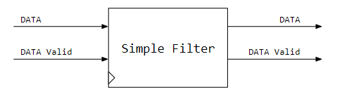
Top level block: 

Nothing too fancy. Data comes in on an enabled line and data comes out the same way. Instead of drawing clock lines, we use the chevron symbol to show that this module is clocked. Our filter needs to run faster than our sampling rate clock so we can run the MAC through our coefficient list before the next sample comes in. The DATA Valid line lets the Simple Filter know that there is a new sample on the line. This enable line should be in sync with the Simple Filter processing clock and we are assuming that the module receiving the sample data is conditioning as such. Now for a closer look inside.

Internals

We are going to use some relatively simple logic elements to build our filter. The table explains each one:

	Addressable Shift Register Samples come in and 10 samples later, they are removed. We can also address this module to get an data from any position in the register on the output.  Clocked.
	Multiplier Multiplies two numbers. We will need to consider bit growth at some point.... Combinatorial
	Adder Adds two numbers. Combinatorial
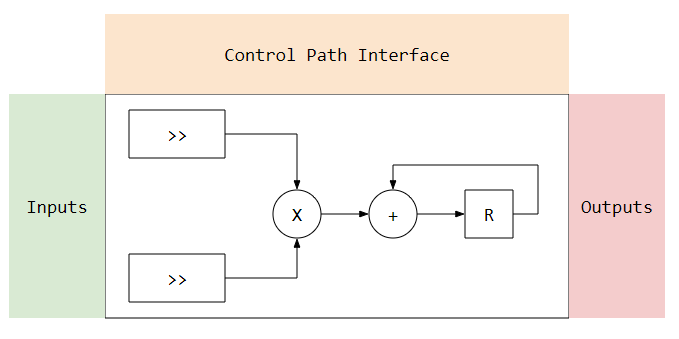
	Register Holds a value of a signal wire. Clocked

Using the elements, we can build a filter below. I have marked the areas I use to diagram up the connections between 3 main areas. 

Inputs, are the inputs from the system into the data path section.

Outputs, are the outputs to the system from the data path section. 

Control Path Interface, is all the controls needed to execute the operations on the data path. 

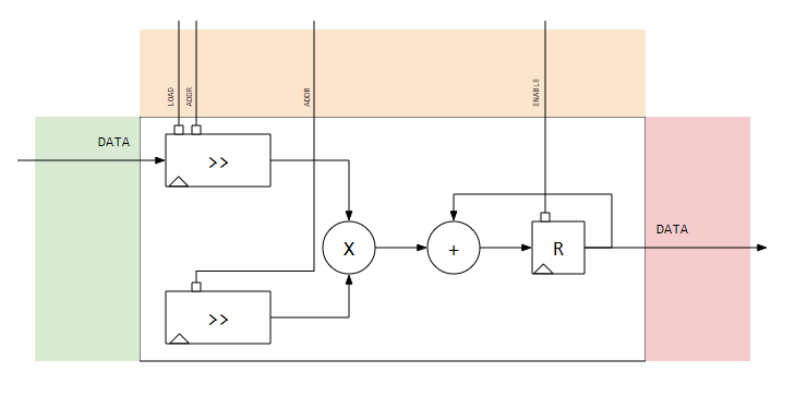
Below shows the connections filled out. 

Notice that the control lines for DATA Valid are not present in this diagram. This signal will be used in the control path section and will help control the signals in the Control Path Interface. 

Conclusions

With the data path processing outlined, we can start thinking about the control path and how we will control the 10 MAC operations in the data path. 

Given that this is a simple design, there are a few glaring issues that will come up. The list includes things like, bit growth from the arithmetic, timing issues from the shift registers to the MAC, and flow control to let the system know we are busy so we don't miss a sample. 

Content taken from a IPython Notebook. Will try and host on Github. 

%matplotlib inline

import matplotlib
import numpy as np
import matplotlib.pyplot as plt

Filter Simulation in Python

The following covers the design and simulation of a filter in python. This code will provide us with the base for running verification in the future. 

Overview

The following is mostly a glossing over of the design process for digital filters. I’m not trying to make this into a filter design how-to, but there are a few things I need to admit up front. 

 - The filter is designed based on a Hamming window.
 - There is no attempt to adjust for added gain

If there is an interest, I can share my process of digital filter design.

Implementation

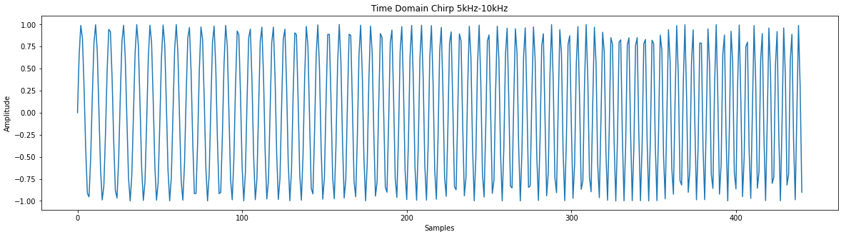
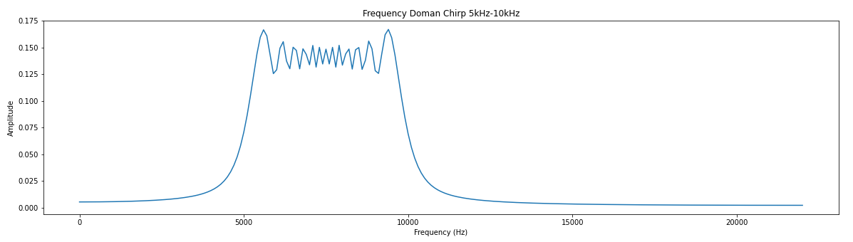
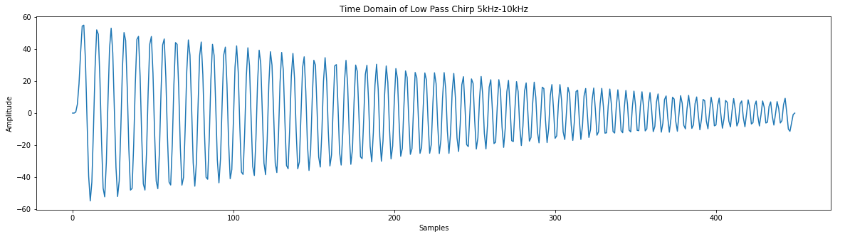
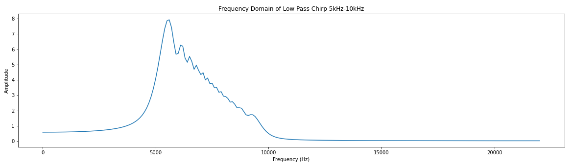
# Low pass filter with a cutoff frequency of 0.1*sample frequency
coeff = [0, 1, 7, 16, 24, 24, 16, 7, 1, 0] # There are larges gains in using this filter 
                                           # We will ignore this for now

# Create a chirp to test with

phi = 0
f0 = 5000.0   # base frequency
f_s = 44100.0  # sample rate (audio rate)
delta = 2 * 3.14 * f0 / f_s
f_delta = 5000 / (f_s * .01)  # change in frequency of 5KHz

s_size = f_s * .01

x = []
for y in range(int(s_size)):
    x.append(np.sin(phi))
    phi = phi + delta
    f0 += f_delta
    delta = 2 * 3.14 * f0 / fs
    
plt.plot(x)
plt.title("Time Domain Chirp 5kHz-10kHz")
plt.xlabel("Samples")
plt.ylabel("Amplitude")

# You might notice the jagged amplitude of the signal. Its aliasing and it sucks.
  

 

# Credit for the easy FFT setup
# https://gist.github.com/jedludlow/3919130

fft_x = np.fft.fft(x)
n = len(fft_x)
freq = np.fft.fftfreq(n, 1/f_s)

half_n = np.ceil(n/2.0)
print(half_n)
fft_x_half = (2.0 / n) * fft_x[:int(half_n)]
freq_half = freq[:int(half_n)]

plt.figure(figsize=(20,5))
plt.plot(freq_half, np.abs(fft_x_half))
plt.title("Frequency Doman Chirp 5kHz-10kHz")
plt.xlabel("Frequency (Hz)")
plt.ylabel("Amplitude")

# Filter implementation
s = np.convolve(x, coeff)  # Real easy

plt.plot(s)
plt.title("Time Domain of Low Pass Chirp 5kHz-10kHz")
plt.xlabel("Samples")
plt.ylabel("Amplitude")

# Results of filter look pretty good. Just the amplitude it way up. 
# We could throw this through a attenuator (divide) to help. 

# Results of the FFT 

fft_x = np.fft.fft(s)
n = len(fft_x)
freq = np.fft.fftfreq(n, 1/f_s)

half_n = np.ceil(n/2.0)
print(half_n)
fft_x_half = (2.0 / n) * fft_x[:int(half_n)]
freq_half = freq[:int(half_n)]

plt.plot(freq_half, np.abs(fft_x_half))
plt.title("Frequency Domain of Low Pass Chirp 5kHz-10kHz")
plt.xlabel("Frequency (Hz)")
plt.ylabel("Amplitude") 

Base Hardware Model

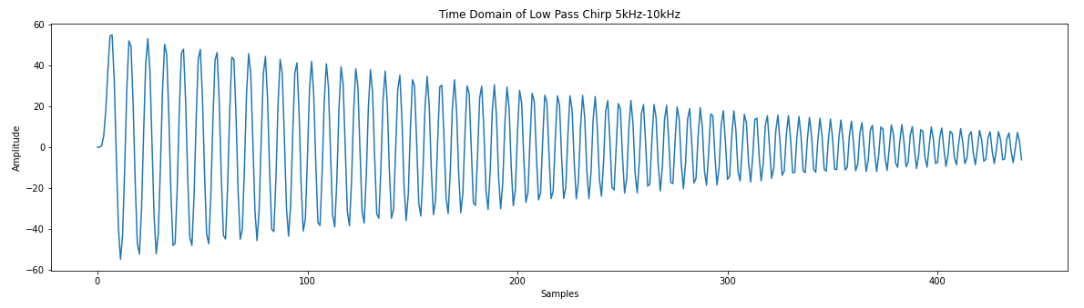
Filter is looking good and we could take these results and test it with our hardware filter later, but lets consider something. While we understand how are filter should perform, we have not yet gained insight to how it should be designed. Lets design a model that shows more of the underlying implementation to help us gain more of an understanding. 

class Filter():
    """ Simple filter model """
    def __init__(self, coeff_list):
        self.coeff = coeff_list
        self.samples = [0]*len(self.coeff)  # Convolution needs a buffer of samples. 
                                            # Unfortunately, the filter will start with 0s
        
    def calc(self, sample):
        ''' Calculate a sample '''
        self.samples.append(sample)  # Samples are loaded from the end
        del self.samples[0]
        return sum([x*y for x, y in zip(self.samples, self.coeff)])  # List comprehension for code brevity.
                                                                     # This is basically what np.convolve does on each sample
            
low_pass = Filter(coeff)

q = [low_pass.calc(x) for x in x]

plt.plot(q)
plt.title("Time Domain of Low Pass Chirp 5kHz-10kHz")
plt.xlabel("Samples")
plt.ylabel("Amplitude")

[EDIT] Conclusions

[EDIT Notes] Looking back through my notes and the data path and control path are pretty closely designed. If anything, the data path is done first and the controls for the data path are decided on afterwards. 

With the base hardware model done, we can start to make some assumptions about what we might need for our control and data path. Such as:

• Computations will take more than one clock cycle and a busy/ready signal would be nice.
• Knowing when the data is valid and invalid
• The ability to load coeff (if wanted) or to hard code the coeff
• Data path will need a multiplier accumulator