Cardware

Shading

Before I can make this model look real I have to do a bit of work regarding how the light falls on it, and it gets a bit complicated because the real one is curved, and the virtual one is made of plane surfaces.

Calculating the path of a beam of light (RayTracing) as it bounces off a surface isnt easy, you need to know the angle of the beam of light, and the angle of the surface, both in 3D. This has to be done after the model is posed for the render, so the only way to know the surface angles for sure is to know their original angles, and back-track the gimballing in the same manner as the leg is calculated.

What, for every pixel? I dont think so... That sounds like hard work. Lets think about it a different way then.

Cloud Theory to the rescue (again)

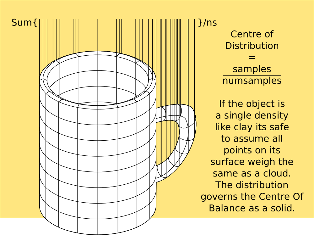
The model is represented as a cloud of atoms with planar surfaces, tiny squares. Each and every one of them has a unique position and angle of incidence, which is calculable, to give the visible area of the model.

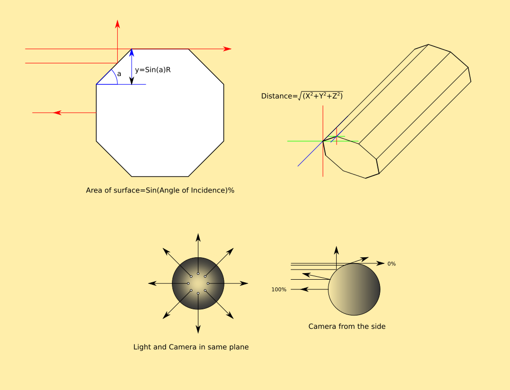
I use IsFacing ( <coords > ) to tell me whether to draw these polygons, because it calculates the area covered by the polygon. If it is negative, it is back-to-front. However, it just returns true or false. If you look at the actual area returned, it is a percentage of its full area when facing the camera directly. When it is sideways-on, it has an area of zero, no matter which way it is facing, left-right or up-down.

This means, by finding the difference between the drawn area and the original, I can tell how much it is facing me without knowing its actual angle, and shade it accordingly.

All polygons facing have 100% area, all polygons side-on have 0% area, and all polygons with -100% area are facing away. This makes it very simple to resolve the shading from the camera, and then rotate the scene to show the shading from another angle.

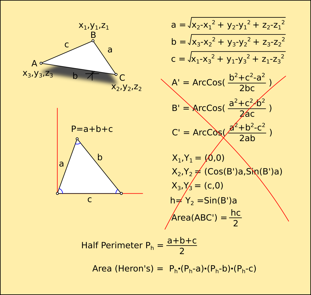
Because it is a rotation, the area and angle are related together by the Sine of the angle. The full area can be calculated by finding the lengths of the sides in 3D, as X,Y,Z offsets as two triangles.

The Law of Cosines could then be applied to give the angles of the sides, and it could be drawn flat without knowing what angle it is facing in any plane...

However, after a bit of digging through my research I realised you can find the area of a triangle much more simply if you know the sides without calculating any angles. Heron's Formula uses the perimeter and ratios of the sides forming it, much nicer. I'd forgotten about that one, usually you wont know all three sides without work so its just as quick to find the height.

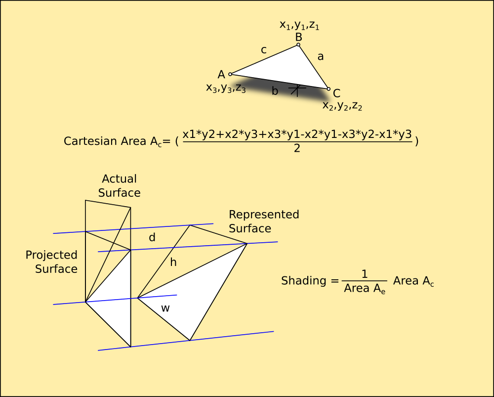
Once it is drawn flat, the area can be calculated as two Euclidean triangles, and the Cartesian Area subtracted from it to give the angle of incidence as a tangent.

The resulting figure is a real value between 0 and 1, giving the amount of atoms visible as a percentage. Because each atom has no height dimension, any atom viewed from the side is not visible, and also covers any atoms behind it so they are no longer visible. This means a 10x10 atom square viewed from the side has an area of 10 atoms; its length or width, because all you can see are the leading 10 atoms on the edge. Viewed from directly facing, it has 100 atoms visible. And at 45 degrees only half of each atom shows behind the atom in front, making the area half.

This means I can calculate how much light falls on any pixel without knowing the angle of the surface it is in, just by calculating how much of it shows. Because I also dont need to know the angle of the light-rays either (they are parallel to the camera axis and therefore zero) I can do this after posing the model, using the information embedded in it as an abstract.

Because each polygon is a rectangle its very easy to graduate the shading across the surface so it appears smoothly curved in two directions instead of planar.

def cartesianarea(crd):
  for n in range(len(crd)-1):           # remove duplicate coordinates
    if len(crd)>n:
      if crd.count(crd[n])>=2: crd.remove(crd[n])
  if len(crd)==3:                       # if there's 3 left
    x1,y1,z=crd[0]                      # pick 1st 3 points
    x2,y2,z=crd[1]
    x3,y3,z=crd[2]
    area=x1*y2+x2*y3+x3*y1-x2*y1-x3*y2-x1*y3 # find triangular area, if its negative its facing down
    return area/2.0                     # return the area
  else: return 0                        # otherwise its not a polygon
  
def euclideanarea(crd):
  global d2r
  for n in range(len(crd)-1):           # remove duplicate coordinates
    if len(crd)>n:
      if crd.count(crd[n])>=2: crd.remove(crd[n])
  if len(crd)==3:                       # if there's 3 left
    x1,y1,z1=crd[0]                     # pick 1st 3 points
    x2,y2,z2=crd[1]
    x3,y3,z3=crd[2]
    a=sqr(((x2-x1)*(x2-x1))+((y2-y1)*(y2-y1))+((z2-z1)*(z2-z1))) # find the lengths
    b=sqr(((x3-x2)*(x3-x2))+((y3-y2)*(y3-y2))+((z3-z2)*(z3-z2)))
    c=sqr(((x1-x3)*(x1-x3))+((y1-y3)*(y1-y3))+((z1-z3)*(z1-z3)))
    p=(a+b+c)/2.0                       # find the perimeter and halve it
    return sqr(p*(p-a)*(p-b)*(p-c))     # return area by herons formula
  else: return 0                        # otherwise its not a triangle

 These work nicely...

c=[[-10,-10,0],[10,-10,0],[-10,10,0]] # make a triangle around 0,0,0
for a in range(0,360,45):             # step through 360 degrees every 45
  d=[]                                # make a container
  for x,y,z in c:                     # go through the coords in c
    d.append(rotate(x,y,z,'x'+str(a)))  # rotate them by a and put them in d
  print 'angle: '+str(a)+' cartesian area: '+str(cartesianarea(d))+' euclidean area: '+str(euclideanarea(d)) # show the results
  
angle: 0 cartesian area: 200.0 euclidean area: 200.0
angle: 45 cartesian area: 141.421356237 euclidean area: 200.0
angle: 90 cartesian area: 3.67394039744e-14 euclidean area: 200.0
angle: 135 cartesian area: -141.421356237 euclidean area: 200.0
angle: 180 cartesian area: -200.0 euclidean area: 200.0
angle: 225 cartesian area: -141.421356237 euclidean area: 200.0
angle: 270 cartesian area: -6.12323399574e-14 euclidean area: 200.0
angle: 315 cartesian area: 141.421356237 euclidean area: 200.0
>>> 

 Rotating triangle c around (0,0,0) always returns its correct area with EuclideanArea, and a ratio of it with CartesianArea, which is negative when facing away.

All I need do is

(1/EuclidianArea)*CartesianArea

  to bring it into the range -1 to 1, with 1 describing the triangle facing towards and -1 facing away.

From Google Translate : Organised Pixels.

Hang on a minute, how'd that get into Latin anyway? :-D

Ever Closer...

The equation governing the shape of the virtual robot now includes every single pixel on it's surface. They are all now vectors in their own right, and after a bit of tinkering with a skins editor, will all be uniquely addressable via a flat image that folds around the mesh. That's drawn using the same bitmap for every panel.

I'm only tinkering at the moment, I'm waiting for one of these to arrive.

Adafruit 12-bit 16 Channel PWM/Servo Shield with I2C interface

Yeah I know, the shame lol. I hate to resort to a shield and one from Adafruit at that, but I'm thoroughly sick of the industry making it impossible to join the various modules it uses together without their glue and platform. Plus the power supply issues were insoluble without them. The amount of servos, plus the fact they sink a quarter-amp each and need 6v meant I can no longer buy the components reliably. The rechargeable batteries run at 3.7V, which is a maddening figure. With two in series you get a little over 7V under load, which will toast a servo but not allow enough overhead for a decent 6V regulator. There are low-drop types, but they dont supply 3 amps, even the SMD ones if you can find them.

I mean, its only a chip, but unless I pay somebody to mount it with a decent power converter and all the headers I cant use it. And the Point Field Kinematics doesnt squeeze into an Atmel 328 alongside the servo sequencer.

I decided to drive the servos straight off the Pi, discovered it only had only one PWM... So I went looking and that was the first thing I encountered. Oh, nuts, I clicked BUY before I thought about it too hard.

Providing the servos run off 3.7V, and I've seen it done, this should work with my existing hardware.

Reading the limb sensors

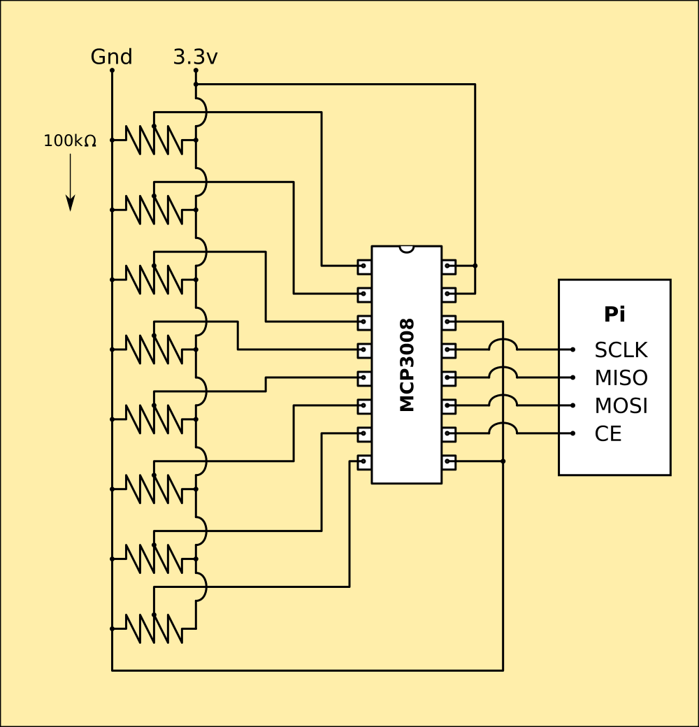
I completely forgot about the potentiometers in the joints... A Pi has no ADC built in unlike the 328, and I need 4 for each limb, 8 in total. Even with a 328 onboard, thats still not enough, and 2 of them seems daft just for their analogue inputs.

I've done a bit of digging to see if there is an ADC I can attach to a GPIO, and Adafruit have one ready made. I can get hold of the chips for that myself, and they use SPI to communicate so that's easy.

MCP3008 - 8-bit 10-channel ADC.

Pretty much plug the chip into the Pi's GPIOs and cable it to the sensors and thats done. Pi has software SPI so I can configure the GPIOs in code. I've ordered one, but it wont arrive until the weekend.

Bummer, I'll just have to polish some pixels until it all arrives.

Mapping is the next big push, mathematically speaking. Luckily I have a head-start on that, I had begun working on it with the original AIME, and have some scrappy code snippets I found randomly on the 'net. I dont know who authored this piece of logic, but they deserve a medal.

bool pinside(poly2d poly, double x, double y) {

  int   i, j=poly.nodes-1;
  bool  oddNodes=false;

  for (i=0; i<poly.nodes; i++) {
    if ((poly.coord[i].y< y && poly.coord[j].y>=y
    ||   poly.coord[j].y< y && poly.coord[i].y>=y)
    &&  (poly.coord[i].x<=x || poly.coord[j].x<=x)) {
      oddNodes^=(poly.coord[i].x+(y-poly.coord[i].y)/(poly.coord[j].y-poly.coord[i].y)*(poly.coord[j].x-poly.coord[i].x)<x); }
    j=i; }

  return oddNodes; }

What it does, is establish whether a point is inside or outside of a complex polygon. Simple polygons are easy, a rectangle particularly so because you can just test it as a matrix. Any cell with a negative index or greater than the width or height is obviously outside. Regular polygons are harder, but still fairly simple - checking the angles of the sides against the line between each corner and the test point to see if they are all larger than that angle is one way of doing it.

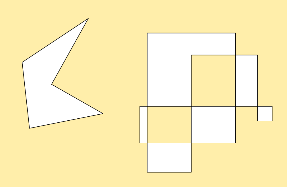
But what about horrible shapes like these (and they will be really easy to create by exploring...)

That second one is particularly nasty. Inkscape has a special routine to handle it in one of several ways depending on how you want it filled. This is default; areas that cross areas already used by the shape are considered outside, unless they are crossed again by a subsequent area. This is how the code snippet interprets a polygon like that, and its useful for making areas from paths for example.

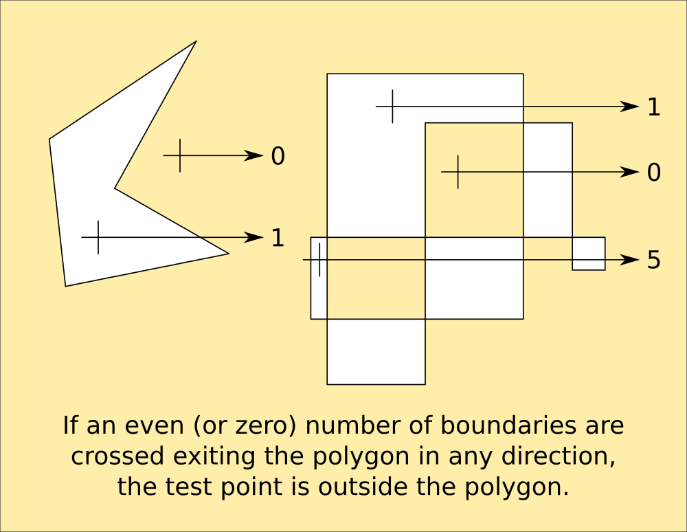
It works by counting the number of boundaries crossed by exiting the polygon from the test point. Obviously a simple regular polygon like a hexagon would return 1 boundary crossed, an odd number of boundaries crossed will always indicate the test point being inside the shape, and an even number of boundaries crossed will indicate outside (providing the crossed-areas rule is observed.)

This is of particular use for sequential-turn mapping of an area, because it identifies the areas enclosed by the path that need exploring, as turns are generated by obstacles that might not be boundaries.

I've finally managed to puzzle out the gimballing for the limbs to the point where I can address them from either end of the chain.

I discovered it wasnt possible to mirror the mesh internally to handle standing on the opposite foot, as I'd planned. It became a nightmare involving such tricks as defining the second mesh inside-out, with anticlockwise polygons, but the gimballing then was reversed too and I gave up, I cant get my head around that.

Instead, I've defined the robot from the left foot, which, when it isnt being stood on, calculates its position backwards from the other foot and then rotates the entire model to make that foot face downwards. Providing all the interstitial rotates are symmetrical, the feet remain parallel to the floor and the sum of the servo angles all add up to 180.

This is highly useful, because it applies with the limbs in a position to step up onto a platform as well as with both of them flat on the floor... Using this information, I've defined a series of poses for the limbs that I can interpolate between and get smooth motion, I've called these seeds, and all the robot's motions will be defined using them.

Here is a full seed set cycled around. I've tilted the display so the part rotates are clearer, but this isnt included in the world coordinate system yet and the position jumps. I'll be refining these, and adding Z rotates for the hips so it can turn. This adds yet another calculation for the far foot position in the mapping system and I'm not there yet.

The next task is to add footprints to the world coordinates, which will enable mapping and platforms, but first I have to integrate the balancing routine and switch that on and off periodically. The seeds are intended to bring the system close to balance, so that I can also use inertial forces later in the development. This will be a matter of timing as well as servo positions; currently I'm working on mapping mode, where it has to determine if there is floor to step onto and thus balance on one foot.

Point Cloud Kinematics

There's actually a lot more to it than meets the eye as far as information is concerned, but it's embedded and bloody hard to get to, because its several layers of integrals each with their own meta-information. I've touched on Cloud Theory before, and used it to solve many problems including this one, but for a cloud to have structure requires a bit of extra work mathematically.

Our universe, being atomic, relies on embedded information to give it form. Look at a piece of shiny metal, its pretty flat and solid, but zoom in on a microscope and you see hills and valleys, great rifts into the surface and it doesnt even look flat any more.

Zoom in further with a scanning electron microscope and you begin to see order - regular patterns as the atoms themselves stack in polyhedral forms.

If you could zoom in further you'd see very little, because the components of an atom are so small even a single photon cant bounce off of them. In fact so small they only exist because they are there, and they are only 'there' because of boundaries formed by opposing forces creating an event horizon - a point at which an electron for example to be considered part of an atom or not. It's an orbital system much like the solar system, its size is governed by the mass within it, which is the sum of all the orbiting parts. That in turn governs where it can be in a structure, and the structure's material behaviour relies upon it as meta-information.

To describe a material mathematically, you then have to also supply information about how it is built - much as an architect supplies meta-information to a builder by using a standard brick size. Without this information the building wont be to scale, even the scale written on the plan. And yet, that information does not appear on the plan, brick size is a meta; information that describes information.

A cloud is a special type of information. It contains no data. It IS data, as a unit, but it is formed solely of meta-information. Each particle in the cloud is only there because another refers to it, so a cloud either exists or it doesnt as an entity, and is only an entity when it contains information. It is self-referential so all the elements refer only to other elements within the set, and it doesnt have a root like a tree of information does.

A neural network is a good example of this type of information, as is a complete dictionary. Every word in the language has a meaning which is described by other words, each of which are also described. Reading a dictionary as a hypertext document can be done, however you'd visit words like 'to', 'and' and 'the' rather a few times before you were done with accessing every word in it at least once. You could draw this map of hops from word to word, and that drawing is the meta-map for the language, it's syntax embedded in the list of words. Given wholemeal to a computer, it enables clever tricks like Siri, which isnt very intelligent even though it understands sentence construction and the meaning of the words within a phrase. There's more, context, which supplies information not even contained in the words. Structure...

This meta-information is why I've applied cloud theory to robotics, and so far it has covered language processing, visual recognition and now balance, and even though the maths is complicated to create it, cloud-based analysis of the surface of the robot is a lot simpler than the trigonometry required to calculate the physics as well.

But its not all obvious...

I first tried to create a framework for the parts to hang off of and immediately ran into trouble with Gimballing. I figured it would be a simple task to assign a series of coordinates from which I could obtain angle and radius information, modify it, and then write it back to the framework coordinates.

This works, and hangs the parts off correctly using the axes to offset each part. To begin with, I just stacked them on top of each other, and then rebuilt that part of the calculation to find the angle the part is at, which worked until I hit the body servos. Working upwards from the foot on the floor, the first servo rotates in the Y axis to tilt the robot back and forwards, and the next tilts it left-and right. Above that another pair of back-and-forwards and above that another left-right tilt. This allows the body to remain parallel to the foot and locate above it in any position within a small circle, so to turn I added a servo to swing the leg around it's axis. This is the one that causes all the trouble, because it changes a left-right tilt into a back-forward tilt as far as the body is concerned, and worse, reverses the other leg completely so a back-forward tilt is a forward-back one.

This is called Gimballing, and its a pain in the arse.

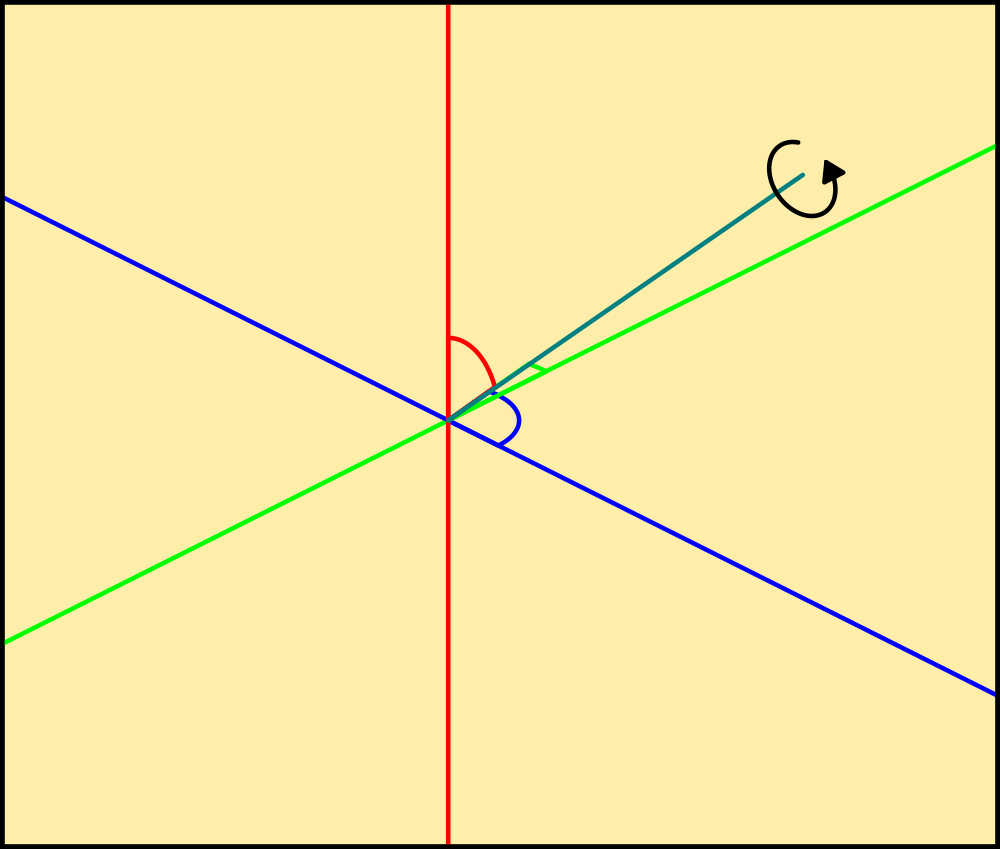
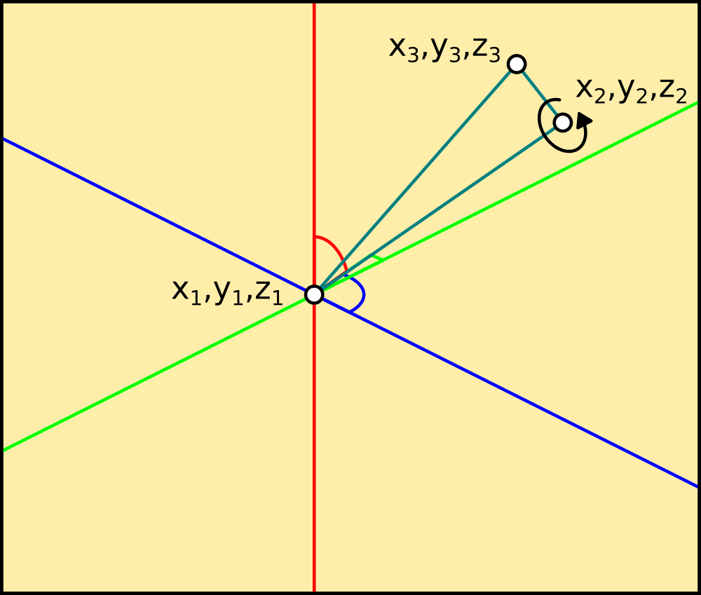
The above drawing illustrates this neatly. X in green, Y in blue and Z in red. The actual angles of the cyan line are specified from the centre as offsets from the axis, so looking along the red line green and blue are a cross and the cyan line rotates around it. The same applies with each axis, but, it doesnt specify rotation around the axis of the cyan line. It's just a line, it needs to have at least another dimension, width or height, before I can tell which way up it is as well as which way its pointing. That gives it an area, a plane surface that contains information about the axis of its edge, which a single line doesnt have.

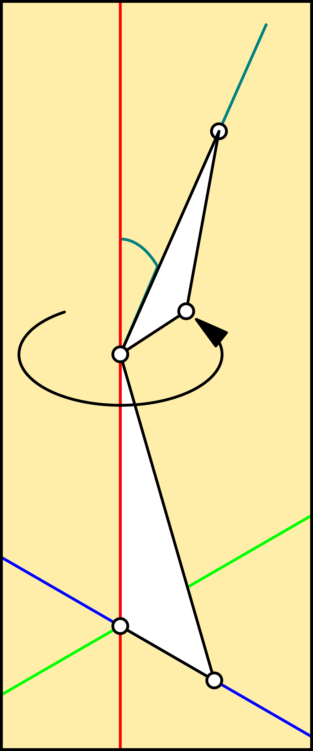
So, each of the joints in the robot has coordinates like this: (XYZ), (XYZ), (XYZ) which each specify a corner of a right-triangle. The Hypotenuse points at the origin at an an angle oblique to the axis which runs along its bottom edge, and the right angle rotates around it, giving it dimension that I can use to locate the top surface of the part - and therefore keep it pointing in the right direction. Cartesian coordinates translate and rotate with respect to each other, so the rotation is done using Pythagorean maths rather than Euclidean, which makes no account of world coordinates like this.

While it isnt immediately apparent, the vertex of the right triangle is the locus for the part, which points at the locus of the next. It is done this way because the very first right triangle sits with it's Opposite on the origin pointing North, and the Adjacent and Hypotenuse point upwards, to meet at the next vertex, which points at right-angles to articulate the joint around the Opposite's axis. This continues up the limb, through the body and out to the free foot.

Assigning a weight to each of those nodes and averaging it across the X-Y plane is enough to balance the entire structure without calculating the limb angles, or computing the entire mesh - although it works with even more accuracy and would be needed with another pair of limbs not in contact with the ground, or non-symmetrical parts. technically this is is cloud sampling rather than cloud analysis, but the end result is the same.

This is all it takes to balance a model using Point Cloud Kinematics.

while not quit:                               # loop forever

  model=[]              # store the models coords as a cloud
  xaverage=[]           # stores all the x coordinates for averaging
  yaverage=[]
 
  for n in range(len(coords)): model.append([0,0,0]) # place all points at the centre

  for n in range(len(mesh)-1,-1,-1):              # begin at the free foot and work down
    for m in mesh[n]:                             # pick up the right coordinates for the part
      for c in m[0]:                              # all 4 corners of the all the polygons
        model[c]=coords[c]                        # transfer them to the model
    for c in range(len(model)):                   # now go through the model points
      x,y,z=model[c]                              # one by one
      s=0                                         # clear last offset position
      if n>0:                                     # if not on the floor
        r=axes[n][0][1][0]+str(axes[n][0][1][1])  # pick up the joints actual positions
        x,y,z=rotate(x,y,z,r)                     # rotate the part around the origin
        s=origins[n][2]-origins[n-1][2]           # move the part +z so it matches the axis
      model[c]=x,y,z+s                            # of the next part below it
  for n in model:
      xaverage.append(n[0])                       # store the modified coords for averaging
      yaverage.append(n[1])

  balance=[sum(xaverage)/len(xaverage),sum(yaverage)/len(yaverage)] # bang, thats the centre 

  if int(balance[0])>1:                           # line up the ankle servo 
    axes[1][0][1][1]=axes[1][0][1][1]+1
    chg=True

  if int(balance[0])<0:
    axes[1][0][1][1]=axes[1][0][1][1]-1
    chg=True
  
  if chg==True:                                   # display the model
    pygame.draw.rect(screen,(255,255,192),((0,0),(1024,768))) # clear the screen
    rend=qspoly(renderise(mesh,model,(cx,cy),'z'+str(ya)+' x'+str(xa),True)) # build the render
    display(rend,'z'+str(ya)+' x'+str(xa))
    chg=False

And other arcane mutterings.

After meeting a dead-end in AIMos with the image recognition based on pixels, I realised I'd have to find a way to either make them triangular to use Euclidean math on them, or, find a way to make Euclidean math work on polygons with 4 sides to match the Cartesian geometry of a photo. Digital images are pretty lazy, just a grid of dots with integer dimensions reduced to a list of colours and a width and height.

It isnt immediately obvious but that isnt how a computer handles a pixel on screen because of scalable resolution. Once inside, it has 4 corners with coordinates 0,0 , 1,0 , 1,1 and 0,1 and happens to be square and the right size to fit under a single dot on the display. The display is designed for this, and modern monitors can even upscale less pixels to give a decent approximation of a lower resolution image.

This interpolation, averaging of values, can also be used to reshape an image by getting rid of the pixels completely, which turned out to be the answer to the problem.

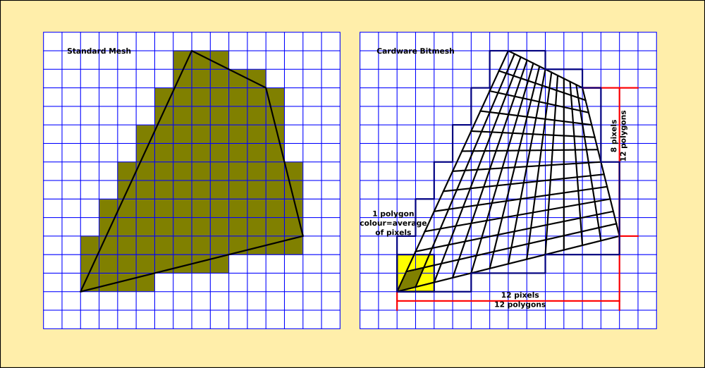
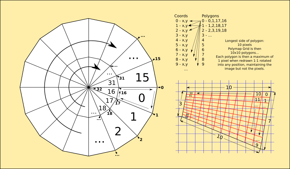
Cardware's internal rendering system hybridises Euclidean and Cartesian geometry to produce a bitmesh, which is a resolution-independent representation of a digital image. It cant improve the resolution of the image, so it works underneath it, using several polygons to represent one pixel and never less than one per pixel.

This is achieved by using the original resolution to set the maximal size of the polygons, and then averaging the colours of the underlaying pixels. Then whenever that polygon is reshaped, it maintains the detail contained in it as well as the detail between it and its neighbours independently of the screen grid. Taking the maximum length of the sides and using that as the numeric base for the averaging does this a lot faster than Fourier, even Fast Fourier routines to abstract and resolve the pixel boundaries.

Because the system now has an abstraction of the image, it can be played with so long as the rules of its abstraction are obeyed. Everything is in clockwise order from out to in, or left-to right and down as per writing, and has logical boundaries in the data that obey Cartesian rules. This means I can use Pythagorean maths, but handled like Euclidean triangles with unpolarised angles that are simply relative to each other.

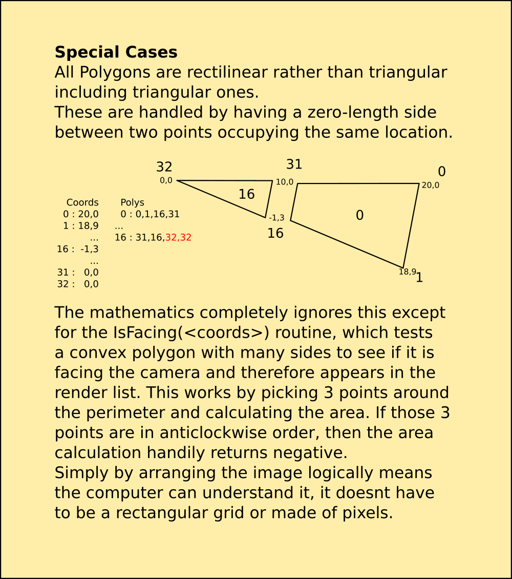
Triangles are unavoidable, but I struck on the idea of making them 4 sided so they handle the same as squares and dont require special consideration. A zero-length side and a zero theta does not interfere with any of the maths I've used so far, and only caused one small problem with an old routine I imported from AIMos. That was easy to write a special case for, and isnt really part of the maths itself, but part of the display routines.

Here's a stalled draw from the Python POC code showing the quality the system can achieve. I was expecting Castle Wolfentstein, but this is going to be more like Halo, near-photographic resolution, and fast too.

The Python that draws this is the calculation routine with pixels obtained from the source map and re-plotted. Once the polymap has been deformed by the mesh and rotated into place those pixels will be polygons and the holes will disappear. The original was 800x600 and takes around 12 seconds to fully render. Once in C++ this will come down to a fraction of a second for a photo quality shell-render of the entire robot, maybe a few frames a second if I'm careful.

Not in a Pi though, so compromises will have to be made...

Yeah I know, walking, I'm not ignoring it.

Actually this maths is all related directly to it as well as the recognition system and the perceptual model I'm trying to build...

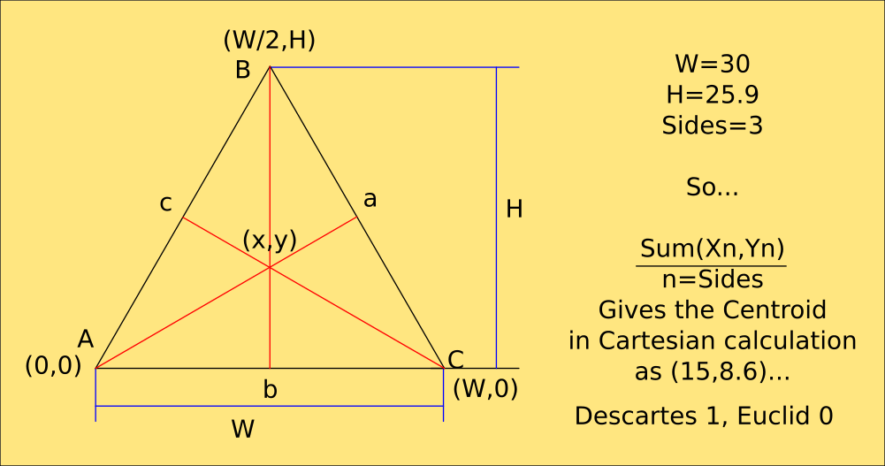
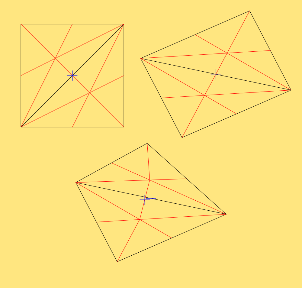
OK so now I know where the actual centre of a triangle is without an awful lot of messing around. That's an equilateral and quite easy to calculate, but a right-angled triangle, of which you find two of in a square will give you two centres if you're using rectilinear shapes. To find the centroid of that you'd need to then calculate the angle and distance between them and halve it to get the true centre, and only if its regular. Using this knowledge can test for regularity of a shape though, which Cartesian math cant as easily.

The last shape is irregular, which can easily be determined from the centroid not being on any line.

Obviously, summing the coordinates of the above shapes as triangles, or as rectinlinear shapes makes no difference because Xn + Xn +Xn / 3 is the same as Xn + Xn + Xn + Xn / 4 and the same with the Y coords.

If you happen to have a Z coordinate too, it will find the centroid of a solid object.

Whats the Centroid anyway, and whats it got to do with anything?

Well, if you take a piece of card and cut an equilateral triangle accurately enough, mark the centre accurately enough and give it a bit of a head-start by curving it slightly, it will balance comfortably on the sharp tip of a pencil.

The Centroid of a plane polygon is its centre of balance, and the Centroid of a polyhedron is its centre of gravity.

Extrapolating that, the Centroid of the Centroids of a group of polyhedrons of equal density then, is the centre of balance for the group, and also the system's LaGrange Point for those interested in orbital mechanics.

And its most easily calculated by summing all the vertices in the model and dividing by the number of them summed. Weight distribution, because the mass of the robot is easily calculable, then becomes a ratio based on the Centroid in any plane and is done without even bothering with the angles of the joints, leaving me free to calculate Gimballing without tortuous trigonometry.

Weight distribution can be calculated directly by assigning ratios of unitary weight to the nodes in the mesh, then the true centre of gravity can be calculated using real-world measurements to back-up what sensor data is telling me. The above model would be very hard to calculate without using the meshcount and vertex distribution along with the meta of them being unitary and therefore equal..

The robot is defined as a chain of angles from floor to free foot through the hips, its just a single line, which is easy to hang the vertex list off of, and calculate weight distribution from independently of movement. The shape of the robot, defined by the corner vertices in relation to the centroids defines the robot's perimeter, which in turn defines its volume and therefore mass by relation to its weight, so the physics model for that is unnecessary, in a strange twist of fortune. I'm just guessing at the ratios for the above drawing, but all I have to do is weigh each real part, and because it is symmetrical assume it is of equal density and assign an nth of the weight to each vertex n and that can calculate the centre of balance in one simple equation, without trig.

Even I'm impressed. :-D

...And populating them

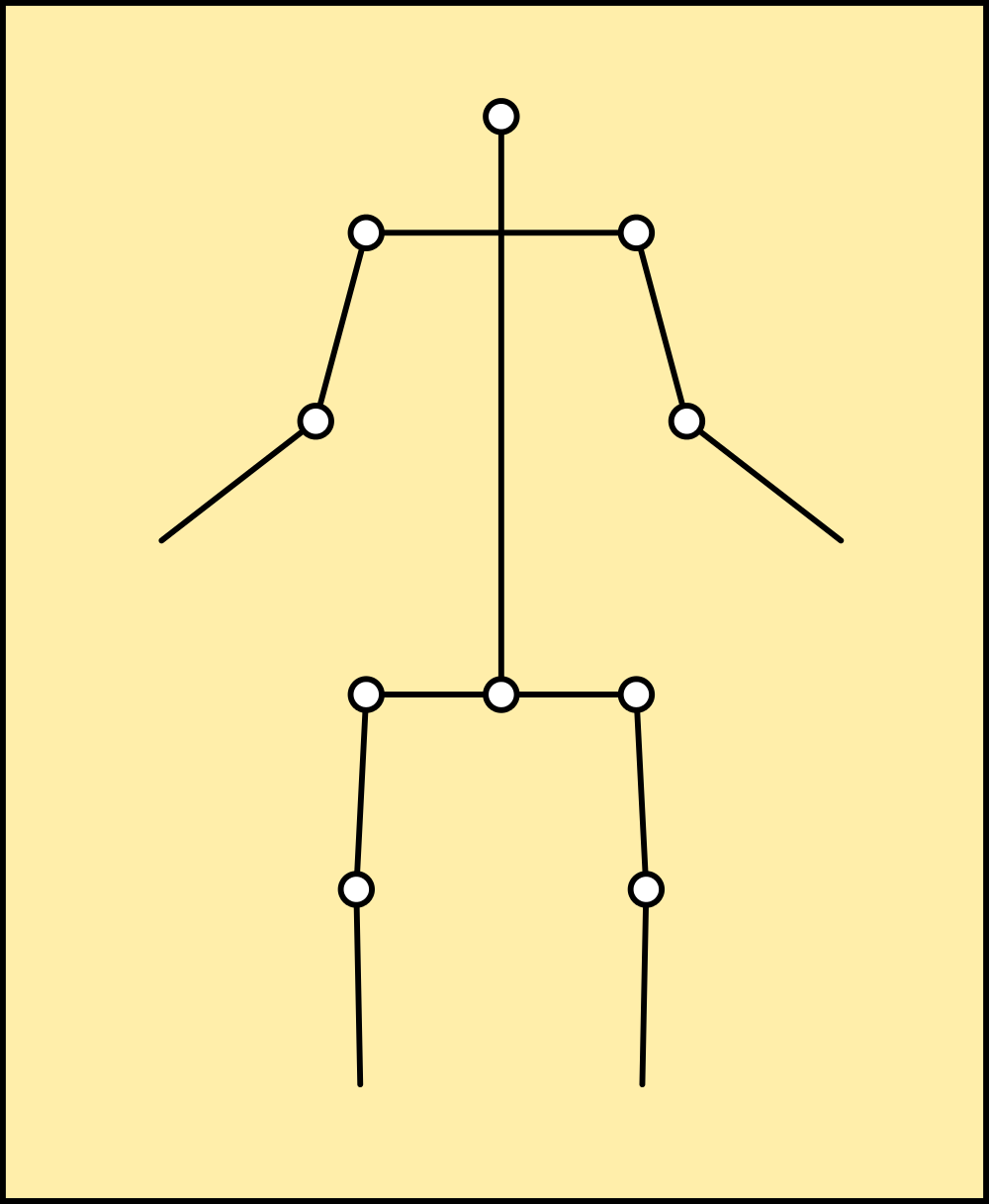
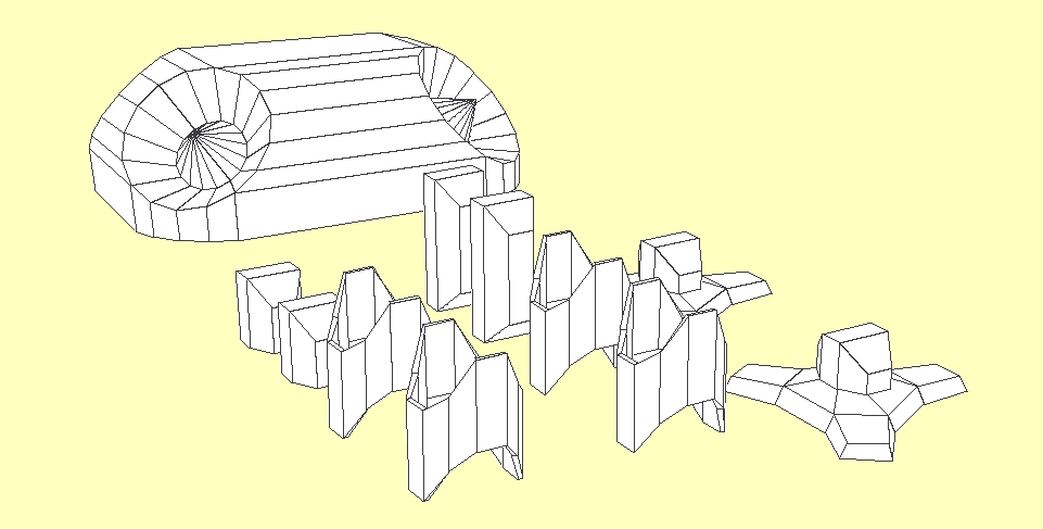
* Now with code to handle multiple objects, save and load objects to a human-readable file and rotate the scene with the cursor keys. This is as about as far as I am taking the Python code as it has served its purpose, to design and assemble the models. There is a bit of tidying up needed, a routine to attach the limbs in a proper chain using the joint angles to display the entire model... And another to export the parts as WaveFront object files, which is pretty easy. Then Cardware can be 3D-printed, milled and rendered in almost any rendering package commercial or otherwise, be simulated in many engines, and, represented by a networked Cardware engine and optionally attached to the sensors on a real Cardware model...

Most of this code will be rewritten in C++ so I can draw those polygons with my own routines and handle the depth on a per-pixel level. This also means I can wrap a photograph of the real one around it. Python is way too slow for this without a library, and PyGame's polygon routines would still be terrible if they understood 3D coordinates. ;-)

I suppose I have to make that skins editor I toyed with while printing the plans now, to make that easy. Double-sided prints are possible but are a bit of a pain to line up properly and I dont have cash for colour cartridges laying around, or at least some of my Metal Minister would have been photographic. Using a skins editor can make that simple, and it isnt just for pretty although that is a consideration;

The main reason is to map the robot's markings to its geometry so it is recognisable to another. Because they are a shared system this information is available to all robots in the network so they can say this is where I am and this is what I look like, so the visual recognition system can verify it and link it to the world math. But, it doesnt have to be a real robot, it can equally be a simulation which the individual robot's 'mind' wont be aware of. Even the simulated ones...

We beep, therefore we are. :-D

To understand the world, and indeed itself, a robot needs to metricate everything and represent it mathematically. It is very important for movement that the robot also understands its perimeters and not just the angles of the joints, so it has situational awareness. So, the first thing I had to do was measure everything and create mathematical models for it to represent itself with.

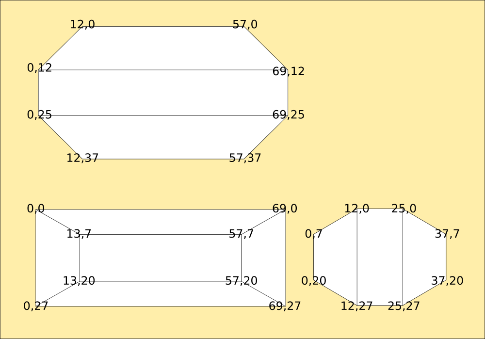
First the easy bits, simple to pull measurements directly off the plans in MM. I'm using that because it fits better into denary math and I can round it to the nearest MM without affecting the shape. The card itself has a 0.5MM width and the physical model can vary by that anyway.

Turns out the model can deviate quite a lot from the plans even when they are printed and folded to make the actual model, and accuracy has little to do with it in practice on some parts. More on that later...

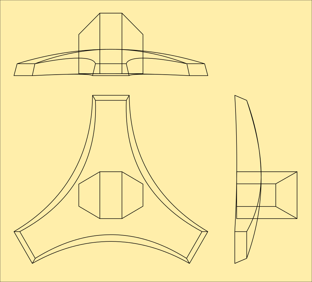
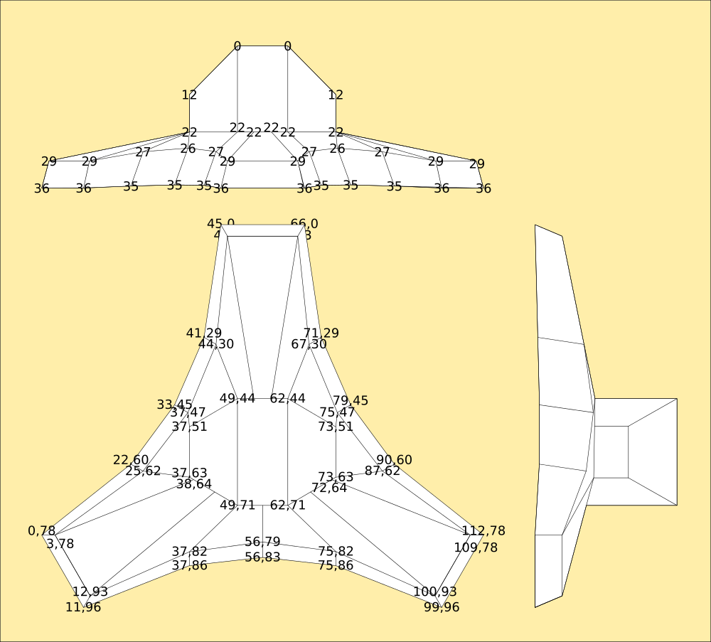
The Thigh Module

Hip and Ankle Modules are simply half of the above part, easy to generate a mesh for during import. The legendary Hip Unit (Units are unpowered, Modules are powered) was already measured to calculate the inner radius from the outer, a 2mm difference in diameter.

The Hip Unit

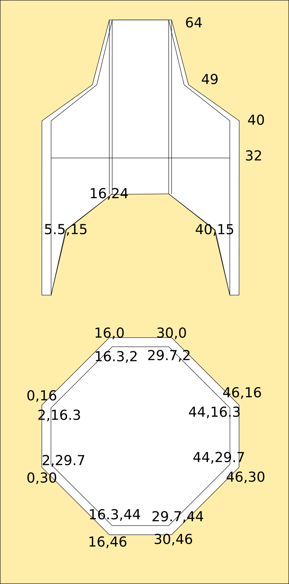
The foot is more complicated. Filled curved shapes are a nightmare to compute edges for, so I've broken them into a mesh. This was done manually in Inkscape from the original drawing.

Overlaid with polygons and then measured, thats the foot done too.

The Foot Module

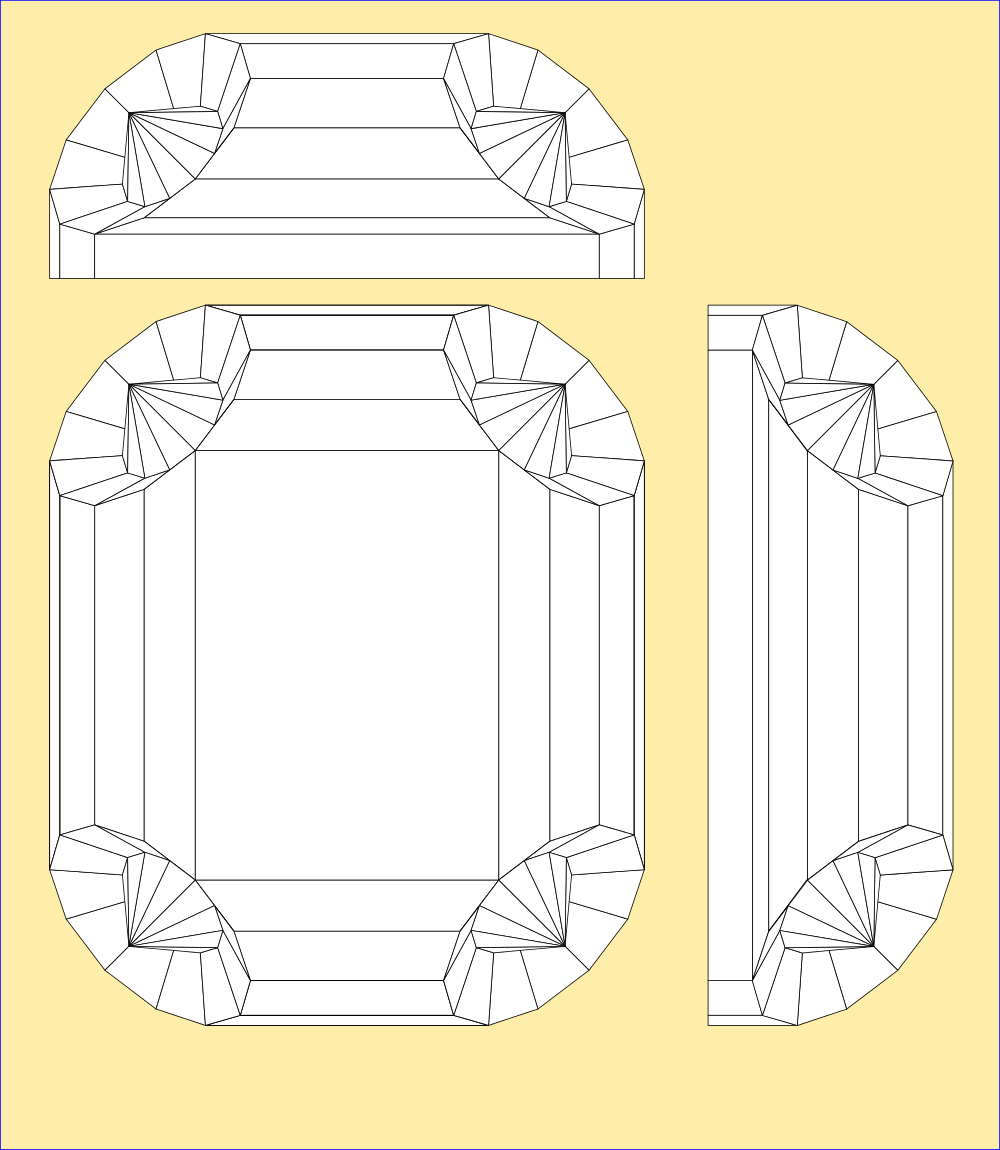
The lid was a little bit more complicated. While I can draw orthogonal plans to scale I'm not entirely sure thats accurate to the MM in all three dimensions. The original MorningStar was not calculated to be the shape it was, I discovered the fold almost accidentally and then figured out the mathematics for it, then used them to compute the lid dimensions as curves. Interpolations from that math was used to create the mesh visually, but is it correct? I dont know for sure.

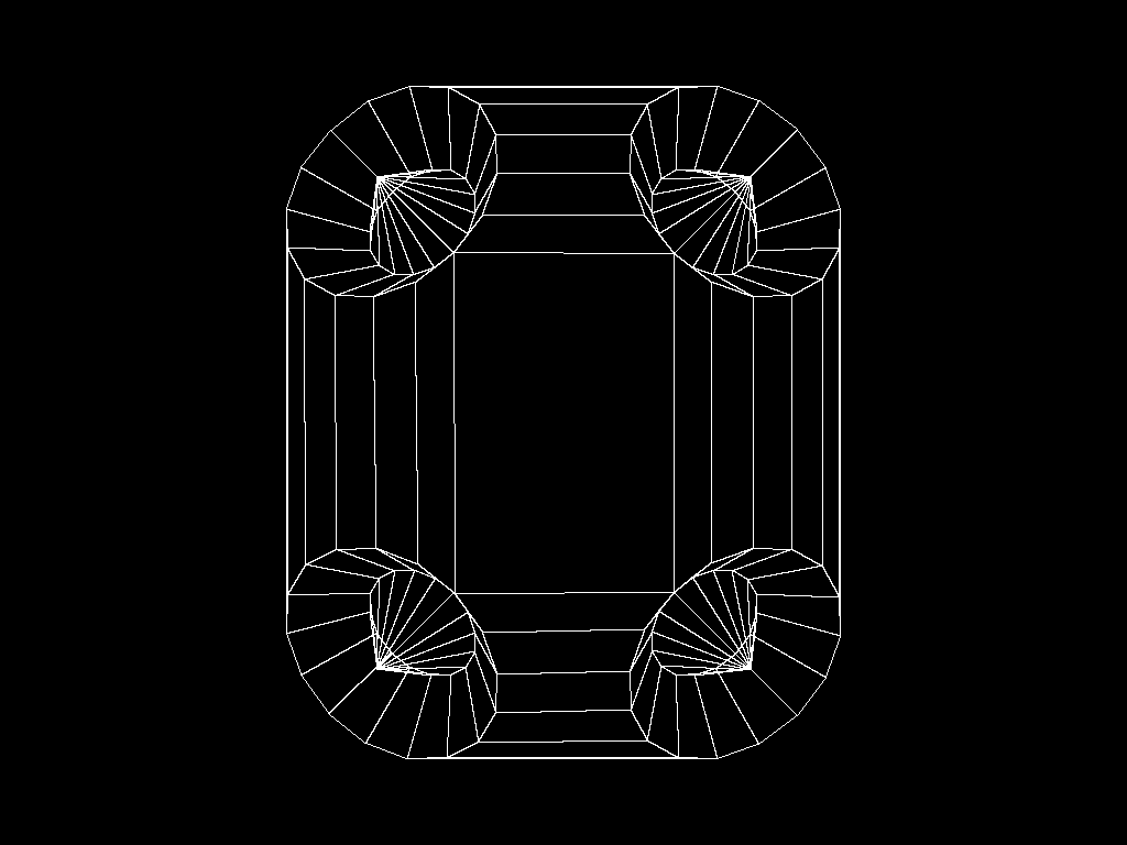
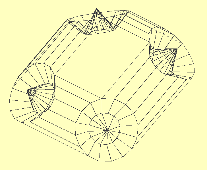
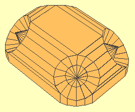
It looks pretty close, but it isnt exact. I recreated the mesh in Python from the given dimensions so I know its accurate. Each corner is defined as 33 points in two concentric circles surrounding a centre point. Then the edges of the circles are joined with polygons.

That just defines the vertices and the edges joining them as a list of XYZ coordinates followed by a list of groups of four pointers into it. Once this information is obtained, its fairly easy to rotate them into any position.

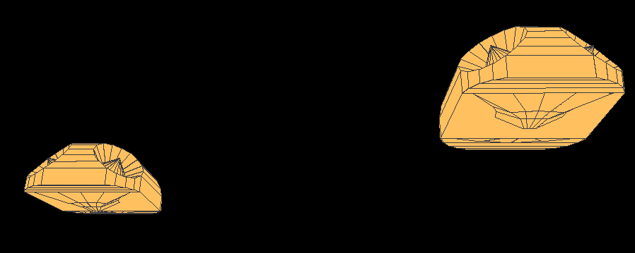
This is still not the end of the story, the computer still doesnt understand 3 dimensions fully although it knows about them. It has to be instructed that the further away from the screen the coordinate is, the smaller it appears - this is perspective projection, and its important because when the robot sees with its camera, the world will be distorted by it and will need correcting for orthogonal projection inside the map.

It also needs to be told that objects can be in front of other objects and thus obscure them, so the system caters for depth by sorting everything it 'sees' into order and working from the back to the front. The computational equation at the end of the log produces this image from just the corner radius and length of the sides between the corners by calculation of all the angles of the polygons mathematically.

The Lid (After a bit of adjusting, to scale. 1px/mm...)

The World

Is mine... Muahahah! Fly, my beauties, fly... XD

Everything the robot experiences will be treated this way. What the camera sees will be projected onto a spherical surface beyond the known meshes, and the meshes are rendered from camera data so the two merge inside the computer memory as a perspective image with embedded 3d information. To crack open intelligence requires creativity, an imagination, so I'm building the robot one that it can perceive the world with rather than just sense it, exactly the same way we do. It produces a render of what it interacts with that can be recreated at any time.

More than this, the robot can render itself and others into a 3d scene accurately because each knows what it looks like and can tell the others. Once experienced, another robot can remember the first down to the pixel and interact with it in imagination, not just real world. Comparing the two should reveal behaviours, which is the purpose of the level of detail I'm using here.

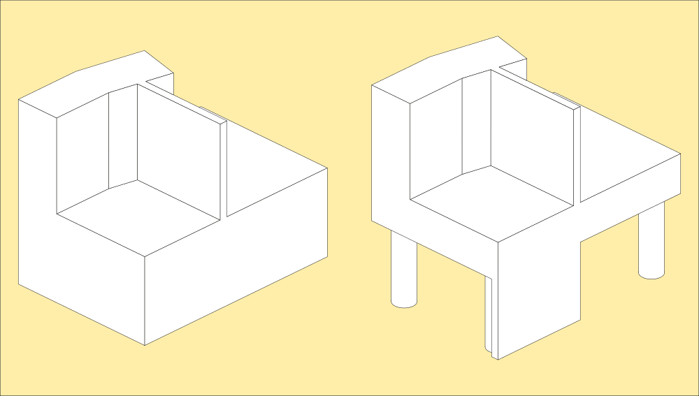
Here is an imaginary representation of a table with a laptop and mouse on it, and a cable across the back. The robot has walked on the first image and mapped the table top but doesnt understand whats under it or around it. The cable is logged as an obstruction, breaking up the surface. I've catered for surfaces by defining the world as a solid until the robot maps it. Anything walked on becomes a flat surface on a pillar, and anything walked under then becomes a floating shelf joined to the ground plane by pillars defined by where it cannot walk. Because the robot will only ever experience things it can walk on or under, and motion in between, it makes assumptions about what is in between and just projects what it can see with its camera on it so it looks like a table.

Understanding of a table then is limited to a surface that can be walked on, above another surface that can be walked on, both with obstructions. Obstructions are treated as pillars with possible walking surfaces on top, but extend to the ceiling unless they are walked on. The robot is equipped with an accelerometer and can estimate height when picked up from the floor and placed on a table.

---

Here is the code used to create the image at the top of the log.

Typically the mathematical model turned out to be too correct; as a full MorningStar the cardboard has to conform to the shape and make 45-degree angles, but cut in half and with extended faces to make a lid it spreads out, explaining a lot of the problems I had with making it fit the base I'd already designed. It seemed simple enough, but I wound up fiddling with the scaling for that a bit. Now I know why, its a few percent bigger than the plan measurement and the correct mathematical model...

Now with edges, which were also a computational nightmare because of the clockwise rule used by the face normalising routines. This complication is necessary, otherwise I'd need an extra parameter in the polygon mesh explaining which direction the face is pointing in. That's encoded into the polygon by listing the corners in clockwise order... All considered, its still simpler than measuring the plans though, and now actually matches the real measurements of the printed and folded one.

In the end, I still didnt have to supply much data to digitise it, and nothing compared to scanning the damn thing, which is the other way of inputting shapes into a computer. This way is elegant and surprisingly simple when you know how - its just a matter of understanding the relationship of the parts to the whole.

from math import sin,cos,atan as atn,sqrt as sqr  # make the maths comfy

import pygame,Image                     # for realtime display
from pygame.locals import *
from time import sleep

pygame.init()                           # set it up
window = pygame.display.set_mode((1024,768))
pygame.display.set_caption("1024x768")
screen = pygame.display.get_surface()

pi=atn(1.0)*4.0                         # pi to machine resolution
d2r=pi/180.0                            # convert between degrees and radians
r2d=180.0/pi                            # and back

### subroutines ###

def test():                             # calculate overall size of entire object in mm
  global coords
  xs=[]; ys=[]; zs=[]                   # temporary lists of x y and z coords
  for c in coords:
    xs.append(c[0])                     # split the lists
    ys.append(c[1])
    zs.append(c[2])
  w=int(max(xs)-min(xs))                # find their bounding box dimensions
  d=int(max(ys)-min(ys))
  h=int(max(zs)-min(zs))
  pygame.image.save(screen,'lidmesh.png') # and dump a bitmap of the current viewport
  xs=[]; ys=[]; zs=[]
  return w,d,h

###

def qspoly(plst):                       # quicksort z coords into order
  lstlen = len(plst)                    # number of polys
  if lstlen <= 1:                       # less than 2 must be in order already
    return plst                         # return it
  elif lstlen == 2:                     # if there's only 2
    if plst[0][0] < plst[1][0]:         # and their z coords are in order already
        return [plst[0],plst[1]]        # return them
    else:                               # otherwise
        return [plst[1],plst[0]]        # swap them
  else:                                 # and return them
    pivpt = plst[0]                     # take the first poly z as a pivot point
    plst1 = []                          # make 2 empty lists
    plst2 = []
    for lstval in range(1,lstlen):      # go through all the z coords
        if plst[lstval][0] < pivpt[0]:  # if the pivotpoint z is greater
            plst1.append(plst[lstval])  # put the poly in one list
        else:                           # otherwise
            plst2.append(plst[lstval])  # put it in the other
    sort1 = qspoly(plst1)               # recursively sort the biggers list
    sort2 = qspoly(plst2)               # and the smallers list
    result = sort1 + [pivpt] + sort2    # then join them all together
    return result                       # and return the list

###
    
def angle(sx,sy):                       # quadratic angle of coords from origin
  if sx<>0: a=float(atn(abs(float(sy))/abs(float(sx)))*r2d) # angle of hypotenuse: arctan(y/x)
  if sx>=0 and sy==0: a=0.0             # point lays on origin or to right; return 0 degrees
  if sx<0 and sy==0: a=180.0            # directly to the left; 180 degrees
  if sx==0 and sy>0: a=90.0             # directly above; 90 degrees
  if sx==0 and sy<0: a=270.0            # directly below; 270 degrees
  if sx>0 and sy>0: a=float(a)          # its in quadrant 1,1; 0.n1-89.9n degrees
  if sx<0 and sy>0: a=float(180-a)      # quadrant -1,1; 90.n1-179.9n degrees
  if sx>0 and sy<0: a=float(360-a)      # quadrant 1,-1; 270.n1-359.9n degrees
  if sx<0 and sy<0: a=float(180+a)      # quadrant -1,-1; 180.n1-269.9n degrees
  return a                              # return actual angle

###

def radius(sx,sy):                      # get radius of coords from origin
  r=float(sqr((abs(float(sx))*abs(float(sx)))+(abs(float(sy))*abs(float(sy)))))
  return r                              # its pythagorus, sum of the root of the squares

def rotate(x,y,z,rs):                   # rotate a point x,y,z around origin 0,0,0
  for ra in rs.split():                 # step through list of rotates
    if ra[0]=='z':                      # z plane
      a=angle(x,y)+float(ra[1:])        # slice the xy plane, find angle and add rotate to it
      r=radius(x,y)                     # find the radius from 0,0,z
      x=cos(a*d2r)*r                    # calculate new x,y,n
      y=sin(a*d2r)*r
    if ra[0]=='x':                      # x plane
      a=angle(z,y)+float(ra[1:])        # slice the yz plane, find angle and add rotate to it
      r=radius(z,y)                     # find the radius from x,0,0
      z=cos(a*d2r)*r                    # calculate new n,x,y
      y=sin(a*d2r)*r
    if ra[0]=='y':                      # y plane
      a=angle(x,z)+float(ra[1:])        # slice the xz plane, find angle and add rotate to it
      r=radius(x,z)                     # find the radius from 0,y,0
      x=cos(a*d2r)*r                    # calculate new x,n,z
      z=sin(a*d2r)*r
  return (x,y,z)                        # return final x,y,z coordinate

###

def isfacing(crd):                      # is polygon facing up (vertices ordered clockwise)
  for n in range(len(crd)-1):           # remove duplicate coordinates
    if len(crd)>n:
      if crd.count(crd[n])>=2: crd.remove(crd[n])
  if len(crd)>=3:                       # if there's at least 3 left
    x1=crd[0][0]; y1=crd[0][1]          # pick 3 spaced equally round the perimeter
    x2=crd[len(crd)/3][0]; y2=crd[len(crd)/3][1]
    x3=crd[(len(crd)/3)*2][0]; y3=crd[(len(crd)/3)*2][1]
    area=x1*y2+x2*y3+x3*y1-x2*y1-x3*y2-x1*y3 # find poly area, if its negative its facing down
    return (area/2>=0)                  # return that, dont need the actual area
  else: return 0                        # otherwise its not a polygon

###

def buildlid(sw,sh,r):
  coords=[]                             # list of vertices
  polys=[]                              # list of polygons
  rot=['z113.5 x50 z45','z22.5 y-50 z45','z292.5 x-50 z45','z202.5 y50 z45'] # corner rotations
  minz=0
  sws=[-((sw/2)+r),(sw/2)+r,(sw/2)+r,-((sw/2)+r)] # width of side between centres of rotation
  shs=[(sh/2)+r,(sh/2)+r,-((sh/2)+r),-((sh/2)+r)] # height of side between centres
  spr=360.0/16                          # spread the points around a full circle

  for s in range(4):                    # make 4 corners
    for a in range(16):                 # with 16 segments each around the edge
      x=cos(a*spr*d2r)*r                # make a circle round the origin
      y=sin(a*spr*d2r)*r                # on the z axis
      z=0                               # on ground plane so origin is at the top
      x,y,z=rotate(x,y,z,rot[s])        # rotate the points in 3d to match the corner angles
      coords.append([x+sws[s],y+shs[s],z]) # add coordinates to vertex list
    for a in range(16):                 # another 16 segments inside
      x=cos(a*spr*d2r)*(r/2)            # make a concentric circle half the size
      y=sin(a*spr*d2r)*(r/2)                 
      z=-r/2.0                          # above the first, again in the z axis
      x,y,z=rotate(x,y,z,rot[s])        # rotate the points in 3d
      coords.append([x+sws[s],y+shs[s],z]) # add coordinates to vertex list
    x=0                                 # make a single point at the centre
    y=0
    z=r/8                               # slightly above the rings
    x,y,z=rotate(x,y,z,rot[s])          # rotate it into place in 3d
    coords.append([x+sws[s],y+shs[s],z]) # add it to the coords list
    if z<minz: minz=z
    
    for n in range(16):                 # now polygons, these point to the actual coords
      a=n; b=n+1; c=n+17; d=n+16        # point at the vertices of ring 1 and 2
      if b>15: b=b-16                   # its a grid; wrap the edges around
      if c>31: c=c-16
      if d>31: d=d-16
      p=[a+(s*33),b+(s*33),c+(s*33),d+(s*33)] # point at correct corner vertices
      polys.append([p,n<16])            # and add the poly to the list
    
    for n in range(16):                 # second ring
      a=n+16; b=n+17; c=n+33; d=n+32    # points at vertices of ring 2 and centre
      if b>31: b=b-16                   # wrap the edges around
      if c>31: c=32
      if d>31: d=32
      p=[a+(s*33),b+(s*33),c+(s*33),d+(s*33)] # point at correct corner vertices
      polys.append([p,n<16])            # add poly to the list
    
  polys.append([[40,7,106,73],True])    # add central square

  for n in range(6):                    # add surrounding polygons between the circles
    polys.append([[7+n,40-n,39-n,8+n],True])      # they are all clockwise
    polys.append([[40+n,73-n,72-n,41+n],True])    # so work out where they are from centre
    polys.append([[73+n,106-n,105-n,74+n],True])
    polys.append([[106+n,7-n,6-n,107+n],True])
    
  lc=len(coords)                        # make a note of the coords to point to
  
  for c in range(4):                    # four corner circles
    for n in range(5):                  # five points intersect with rim
      v=n                               # but they arent arranged in a decent order so
      if n>1: v=n+11                    # bodge the order of the points in the sector
      ev=v+(c*33)                       # for each corner
      x,y,z=coords[ev]                  # find the actual coordinates
      coords.append([x,y,minz-50])      # copy the rim coordinates lower to make an edge
  
  rim=[[1,0,0,1],[0,15,4,0],[15,14,3,4],[14,13,2,3]] # bodge the new rim coordinates to the old ones
  for a,b,c,d in rim:                   # pick up a set of corners
    polys.append([[a,b,lc+c,lc+d],True]) # and make a polygon from them
    polys.append([[a+33,b+33,lc+c+5,lc+d+5],True]) # echo for the other corner pieces
    polys.append([[a+66,b+66,lc+c+10,lc+d+10],True])
    polys.append([[a+99,b+99,lc+c+15,lc+d+15],True])
  
  polys.append([[13,34,lc+6,lc+2],True]) # and fill in the gaps to make complete sides
  polys.append([[46,67,lc+11,lc+7],True])
  polys.append([[79,100,lc+16,lc+12],True]) # bodge...
  polys.append([[112,1,lc+1,lc+17],True])
  
  polys.append([[lc+12,lc+16,lc+15,lc+13],True])    # bridge across the front edge to close the base
  polys.append([[lc+13,lc+15,lc+19,lc+14],True])    
  polys.append([[lc+14,lc+19,lc+18,lc+10],True])    
  polys.append([[lc+10,lc+18,lc+17,lc+11],True])    

  polys.append([[lc+11,lc+17,lc+1,lc+7],True])      # fill in the middle


  polys.append([[lc+7,lc+1,lc+0,lc+8],True])        # and bridge across the back to close that too
  polys.append([[lc+8,lc+0,lc+4,lc+9],True])    
  polys.append([[lc+9,lc+4,lc+3,lc+5],True])        # bodge...
  polys.append([[lc+5,lc+3,lc+2,lc+6],True])
  
  lc=len(coords)                        # make a note of the coords to point to
  
  c=[]                                  # make containers to hold some measurements
  c.append([[78,74,0],[78,74,0],[39,85,0],[0,90,0],[-39,85,0],[-78,74,0],[-78,74,0]])    # behold my shiny
  c.append([[48,34,0],[30,41,10],[14,44,10],[0,45,10],[-14,44,10],[-30,41,10],[-48,34,0]]) # quadratic
  c.append([[42,18,0],[16,25,12],[9,25,12],[0,26,12],[-9,25,12],[-16,25,12],[-42,18,0]])  # metal
  c.append([[39,0,0],[7,0,14],[3,0,14],[0,0,14],[-3,0,14],[-7,0,14],[-39,0,0]])       # ass-plate bodge ;)

  for a in range(4):                    # iterate the containers
    for n in range(7):                  # iterate the vertices in the containers
      x,y,z=c[a][n]                     # make the top half
      coords.append([-x,y,minz-50-z])   # and write it into the coords pool
  for a in range(3,0,-1):               # make the bottom half
    for n in range(7):
      x,y,z=c[a-1][n]
      coords.append([-x,-y,minz-50-z])  # write it to the pool
      
  for t in range(6):                    # 7 rows of vertices, 6 columns of polys
    for n in range(6):                  # 7 columns of vertices
      polys.append([[lc+n+(t*7),lc+n+(t*7)+1,lc+n+(t*7)+8,lc+n+(t*7)+7],True]) # write the polys

  return polys,coords                   # and return the complete orthogonal set

###

def renderise(msh,verts,ctr,agl):       # build a list of 2d polygons from 3d data
  global origins,scl                    # pick up the positions of the objects
  render=[]                             # make a blank scene
  for i in range(len(mesh)):            # go through all the objects
    for m in msh[i]:                    # go through all the polys in the object
      az=0                              # centroid position
      crd=[]                            # blank list of 2d coordinates for pygame.draw.poly()
      for c in range(4):                # 4 corners for hybrid 'bitmesh' polygons
        x,y,z=verts[m[0][c]]            # get the coordinates of the corners
        x=x+origins[i][0]
        y=y+origins[i][1]
        z=z+origins[i][2]
        x,y,z=rotate(x,y,z,agl)         # rotate them into 3d space
        persp=(z+1000)/1000.0           # calculate perspective distortion
        x=x*persp*scl; y=y*persp*scl    # and apply it to each vertex
        crd.append([x+ctr[0],y+ctr[1]])
        az=az+z
      az=az/4.0                         # find the average z of the four (the centroid)
      if isfacing(crd):                 # if its facing towards camera (up or +z)
        render.append([az,crd])         # render it
  return render

def savemesh(fil,i):                    # save the submesh as a modified wavefront format file
  global mesh,coords,origins,axes       # pick up the entire set
  f=open(fil,'w')                       # make a file
  f.write('#cardware object\n\n')       # make a header
  f.write('#parameters\n')              # write out metadata
  for n in range(len(axes[i])):         # angles of the legs are held in a chain from foot to foot
    f.write('a '+str(axes[i][n][0])+','+str(axes[i][n][2][0])+','+str(axes[i][n][2][1])+','+str(axes[i][n][2][2])+'\n')
  f.write('\no '+str(origins[i][0])+','+str(origins[i][1])+','+str(origins[i][2])+'\n')
  f.write('\n#vertices\n')              # write out vertex data
  minp=mesh[i][0][0][0]
  maxp=mesh[i][0][0][0]                 # first polygon corner vertex in submesh
  for p in mesh[i]:                     # find the all others
    for m in p[0]:
      if m<minp: minp=m                 # determine the range within the coords block
      if m>maxp: maxp=m
  print minp,maxp
  for c in range((maxp-minp)+1):        # select just submesh vertices from the master vertex list
    x,y,z=coords[c+minp]
    f.write('v '+str(x)+', '+str(y)+', '+str(z)+'\n') # and write them to the file
  f.write('\n#faces\n')
  for p in mesh[i]:                     # now go through polygons pointing to those vertices
    a,b,c,d=p[0]                        # pick up the corner vertices
    if p[1]:                            # write out the modified vertex pointers
      f.write('f '+str(a-minp)+', '+str(b-minp)+', '+str(c-minp)+', '+str(d-minp)) # if its drawn write the polygon
    else:                                                                          # otherwise
      f.write('#f '+str(a-minp)+', '+str(b-minp)+', '+str(c-minp)+', '+str(d-minp)) # just annotate it in the file
    f.write('\n')
  f.close()
  
def loadmesh(fil,i):                    # load a mesh into the coord and polygon blocks
  global mesh,coords,axes,origins,cx,cy # pick up mesh structures
  imesh=[]; icoords=[]; iaxes=[]; iorigs=[] # make new blank ones
  lc=len(coords)                        # make a note of the current vertex list length
  f=open(fil,'r')                       # open the file
  lst=list(f)                           # load it into a list
  f.close()                             # close the file
  icx=cx; icy=cx; icz=0                 # new instance defaults to screen center
  minx=0; miny=0; minz=0
  maxx=0; maxy=0; maxz=0
  if '#cardware object\n' in lst:       # make sure its a cardware mesh
    err=False                           # check syntax
    centre=False                        # use quadratic cartesian coordinates
    for l in lst:                       # go through lines one by one
      if l.strip()!='':                 # if its not a blank line
        if '#' in l: l=l.strip().split('#')[0].strip() # remove annotations
        if l>'':                        # if its still not blank
          if l[0]=='v':                 # if its a vertex line
            l=l[1:].strip().split(',')  # remove the preamble and snap it at commas
            x=float(l[0])               # and read it as three floating point values
            y=float(l[1])
            z=float(l[2])
            if x<minx: minx=x
            if y<miny: miny=y
            if z<minz: minz=z
            if x>maxx: maxx=x
            if y>maxy: maxy=y
            if z>maxz: maxz=z
            icoords.append([x,y,z])     # store it temporarily
          elif l[0]=='f':               # otherwise, if its a face line
            l=l[1:].strip().split(',')  # snap it at commas
            a=int(l[0])+lc              # read the pointer and modify it to point past
            b=int(l[1])+lc              # the existing coords
            c=int(l[2])+lc
            d=int(l[3])+lc
            imesh.append([[a,b,c,d],True]) # store it temporarily
          elif l[0]=='o':               # otherwise if its an origin; initial position in map
            l=l[1:].strip().split(',')  # snap it up
            icx=float(l[0])             # and make a note of it
            icy=float(l[1])
            icz=float(l[2])
          elif l[0]=='a':               # otherwise if its an articulation
            l=l[1:].strip().split(',')  # snap it up
            a=int(l[0])                 # get the id of the part and articulation it attaches to
            x=float(l[1])               # and the relative coords of the centre of rotation
            y=float(l[2])
            z=float(l[3])
            iaxes.append([a,[0,0,0],[x,y,z]]) # temporarily store the id, angles and position
          elif l[0]=='c':               # otherwise is a flag to say data is topleft or quadratic
            centre=True
          else:                         # otherwise its not supposed to be there
            print'** warning ** malformed file **'
            err=True                    # so give up on load without modifying memory
            
  else:
    print '** not a cardware file **' # otherwise, cant even see a proper format
    err=True

  if not err:                           # providing all went to plan
    while len(mesh)<=i:
      mesh.append([])
      axes.append([])
      origins.append([])
    for c in icoords:
      x,y,z=c
      if centre:
        x=x-((maxx-minx)/2.0)
        y=y-((maxy-miny)/2.0)
        z=z+((maxz-minz)/2.0)
      coords.append([x,y,z])  # append the new coords to the end of the coord block
    for p in imesh: mesh[i].append(p)   # add the new polygon pointers to the mesh block
    for a in iaxes: axes[i].append(a)   # attach the new part to the parts chain
    origins[i]=[icx,icy,icz]            # and give it an initial reference position
    
### main routine ###

cx=512; cy=384                          # centre coords of screen
r=43; sw=25; sh=80                      # morningstar template radius, side lengths
render=[]

coords=[]
mesh=[]
axes=[]
origins=[]

#msh,coords=buildlid(sw,sh,r)           # build the lid
#mesh.append(msh)
#savemesh('body.msh',0)

loadmesh('body.msh',0)
loadmesh('thigh.msh',1)
loadmesh('thigh.msh',2)
loadmesh('hipmodule.msh',3)
loadmesh('hipmodule.msh',4)
loadmesh('hipunit.msh',5)
loadmesh('hipunit.msh',6)
loadmesh('hipunit.msh',7)
loadmesh('hipunit.msh',8)
loadmesh('foot.msh',9)
loadmesh('foot.msh',10)

origins[0]=[-300,0,30]
origins[1]=[-100,0,0]
origins[2]=[-50,0,0]
origins[3]=[-100,100,-17]
origins[4]=[-50,100,-17]
origins[5]=[25,0,0]
origins[6]=[100,0,0]
origins[7]=[25,100,0]
origins[8]=[100,100,0]
origins[9]=[-100,-150,0]
origins[10]=[50,-150,0]

chg=False                               # display changed flag
xa=-90                                    # rotation of entire scene round origin
ya=0
scl=2.0

rend=qspoly(renderise(mesh,coords,(cx,cy),'z'+str(ya)+' x&ap

Well, finally I was let down by a lack of amps, the batteries I have just arent strong enough to move the limbs without at least doubling them. And I'll need to upgrade the regulators. Such is life...

I added a little bit of code to the Pi's monitor. The raw_input() function was going to be replaced by an open() and list() on a script containing mnemonics.

def injector():
  global port,done,packet
  
  print 'Starting input thread.'
  
  joints=['anklex','ankley','knee','hipx','hipz']
  cmds=['movs','movm','movf','movi']
  syms=['s','m','f','i']
  rngs=[15,10,5,1]
  while not done:
    cmd=-1
    spd=-1
    srv=-1
    agl=-1
    print '->',
    i=raw_input('')
    if i!='':
      inp=i.split(' ')
      if len(inp)==3:
        srv=0
        if inp[0] in cmds: cmd=cmds.index(inp[0])
        if inp[1] in joints: srv=joints.index(inp[1])+1
        try:
          agl=int(inp[2])
        except: agl=-1
        if cmd>-1:
          spd=rngs[syms.index(cmds[cmd][3])]
        if cmd>-1 and srv>-1 and agl>-1 and spd>-1:
          checksum=1+srv+agl+spd # int(i1)+int(i2)+int(i3)+int(i4)+int(i5)
          chk2=(checksum & 65280)/256
          chk1=(checksum & 255)
          port.write(chr(chk1)+chr(chk2)+chr(1)+chr(srv)+chr(agl)+chr(spd)+chr(0))
          sleep(1)
    else: done=True

This would allow me to program motions for the servos, if they actually moved. They hum, but they just dont have the juice.

Closing existing port... Port not open
Clearing buffers...
Connected!
Starting input thread.
-> movm knee 255
Servo: 10 10 128
Move: 10 128
Move: 9 140
Move: 8 153
Move: 7 166
Move: 6 178
Move: 5 191
Move: 4 204
Move: 3 216
Move: 2 229
Move: 1 242
-> movm knee 128
Servo: 10 10 255
Move: 10 255
Move: 9 242
Move: 8 229
Move: 7 216
Move: 6 204
Move: 5 191
Move: 4 178
Move: 3 166
Move: 2 153
Move: 1 140
-> movm anklex 0
Move: 10 128
Move: 9 115
Move: 8 102
Move: 7 89
Move: 6 76
Move: 5 64
Move: 4 51
Move: 3 38
Move: 2 25
Move: 1 12
-> movm anklex 128
Move: 10 0
Move: 9 12
Move: 8 25
Move: 7 38
Move: 6 51
Move: 5 64
Move: 4 76
Move: 3 89
Move: 2 102
Move: 1 115
-> movm anklex 255
Move: 10 128
Move: 9 140
Move: 8 153
Move: 7 166
Move: 6 178
Move: 5 191
Move: 4 204
Move: 3 216
Move: 2 229
Move: 1 242
-> movi anklex 128
Move: 1 255
-> movi anklex 0
Move: 1 128
-> movs anklex 0
Move: 15 0

 This is the above code interacting with a live processor controlling the servos. For now I have just defined the following instructions.

• MOVI - Move Instant; sets the servo angle to the destination in one step.
• MOVS, MOVM and MOVF - Move Slow, Medium, Fast; sets the servo to the position specified interpolating by decreasing numbers of steps.
• The servos are specified by name, AnkleX and AnkleY, Knee, HipY and HipZ, and angle is specified directly as an 8-bit number between 0 and 255.

These execute over time inside the Atmel without further instruction, freeing up the ports and main processor for the task of observing the sensors and interjecting to compensate. It isnt ideal, but it is a lot faster than trying to directly control the servos over those serial links.

I'm going to take a little break from this for a while. Or I will begin to dislike it... And I need to paint, and play my guitar some to chill out.

OK so I've had a good cuss at those rotten processors. Other than commenting that 'Well, I think MOST of them worked when we packed them...' just isnt good enough when money changes hands over it I'm done with them.

Maybe I'll come back to them later along with the multiprocessor networking, when I've had a break...

Meantime, fuelled by panic and a weak but nonetheless calming solution of Ethyl, I rewired the processor board after snapping off and junking the ESP partition. I had to do this, I could not get either of the two ATMega 1284P-PU chips to program. One's in a Sanguino with Sprinter installed on it, I did that myself so I know its good. Except it isnt. I wasted an hour or two on it and that followed the ESP onto the pile of failed crap I paid money for. Four Duinos and two ESPs, a handful of voltage dividers and a few chips just lately.

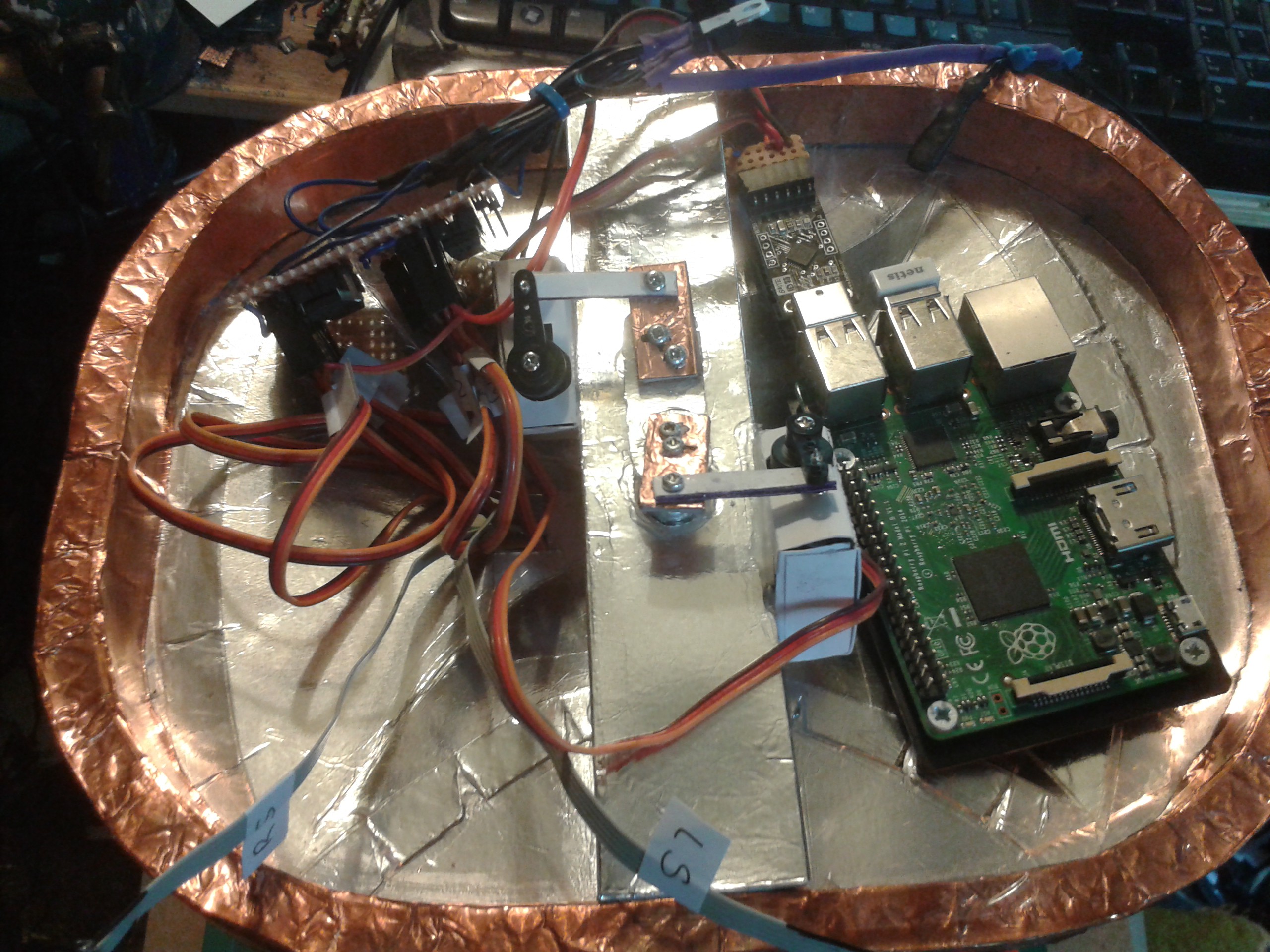
Oh well trusty ATMega 328P-PU's it is then. Each has its own UART and the control code on the Pi talks to the processor via the USB ports, leaving one spare for camera and one for WiFi dongle. There is the option of putting a precompiled solution on the ESP and interfacing to it via the Pi's 40-way connector using #pi2wifi .

Thats now operational and contains a working servo sequencer.

I have managed to rewrite the multicore_ini code to interface directly with the PC and got it working.

#include <Servo.h> 
const int host=1;                                 // this processor
const int servos=5;
// servo definition structure:
// articulation
//      |____ servo (servo object)
//      |          |____ attach()
//      |          |____ write()
//      |____ pin (physical pin number)
//      |____ min (minimum range of movement 0-255)
//      |____ max (maximum range of movement 0-255)
//      |____ home (home position defaults to 128; 90 degrees)
//      |____ position (positional information)
//                 |____ next (endpoint of movement)
//                 |____ pos (current position as float)
//                 |____ last (beginpoint of movement)
//                 |____ steps (resolution of movement)
//                 |____ step (pointer into movement range)
//
// packet configuration:
// byte 1: header - 2 bytes checksum
// byte 2: control - 1 byte packet type
// byte 3: parameters - 1 byte meta
// byte 3: data 1 - arbitrarily assigned
// byte 4: data 2 - arbitrarily assigned
// byte 5: data 3 - arbitrarily assigned
struct servo_position {                           // servo status
  int next;
  float pos;
  int last;
  int steps;
  int step;
} ;
typedef struct servo_position servo_pos;          // atmel c++ curiosity, substructs need a hard reference
struct servo_definition {                         // servo information
  Servo servo;
  int pin;
  int min;
  int max;
  int home;
  servo_pos position;
} ;
typedef struct servo_definition servo_def;        // servo structure containing all relevant servo information
servo_def articulation[servos];                   // array of servo structures describing the limb attached to it
int mins[]={ 0,0,0,0,0,0,0,0,0,0,0,0 };           // defaults for the servo ranges and positions
int maxs[]={ 255,255,255,255,255,0,0,0,0,0,0,0 };
int homes[]={ 128,128,128,128,128,0,0,0,0,0,0,0 };
unsigned char check,checksum,chk1,chk2,ctl,prm,b1,b2,b3;
void setup() {
  Serial.begin(115200);
  while (!Serial) { ; }                           // wait for the port to be available
  for (int s=0; s<servos; s++) {                  // iterate servos
    articulation[s].servo.attach(s+2);            // configure pin as servo
    articulation[s].pin=s+2;                      // echo this in the structure
    articulation[s].home=homes[s];                // configure the structure from defaults
    articulation[s].min=mins[s];
    articulation[s].max=maxs[s];
    articulation[s].position.next=homes[s];
    articulation[s].position.pos=homes[s];
    articulation[s].position.last=homes[s];
    articulation[s].position.steps=0;
  }
  
    for (int d=0; d<1000; d++) {                    // garbage clear
      if (Serial.available() > 0) { unsigned char dummy=Serial.read(); }
      delay(1);
    }  
} 
void loop() { 
  if (Serial.available() >= 7) {                  // if there is a packet
    chk1=Serial.read();                          // read the packet
    chk2=Serial.read();
    ctl=Serial.read();
    prm=Serial.read();
    b1=Serial.read();
    b2=Serial.read();
    b3=Serial.read();
    checksum=chk1+(chk2*256);
    check=ctl+prm+b1+b2+b3;
    if (checksum!=check) { 
      Serial.write(255);
    } 
    
    if ((int)ctl==1) {  // servo instruction
      int agl=(int)b1; 
      int st=(int)b2;
      articulation[(int)prm].position.last=articulation[(int)prm].position.pos;
      articulation[(int)prm].position.next=agl;
      articulation[(int)prm].position.steps=st;
      articulation[(int)prm].position.step=st;
      Serial.write(64);
//      Serial.write(prm);
      Serial.write((int)articulation[(int)prm].position.step);
      Serial.write((int)articulation[(int)prm].position.steps);
      Serial.write((int)articulation[(int)prm].position.pos);
//      Serial.write(st);
    }
    if ((int)ctl==2) {                      // if its a sensor data request send a sensor packet
      int byte1=analogRead(A0)/4;  
      int byte2=analogRead(A1)/4;  
      int byte3=analogRead(A2)/4;
      Serial.write(128);                     
      Serial.write((int)analogRead(A0)/4); 
      Serial.write((int)analogRead(A1)/4);
      Serial.write((int)analogRead(A2)/4);
    }
    if ((int)ctl==4) {
      Serial.write(16);
      Serial.write((int)prm);
      Serial.write((int)articulation[(int)prm].position.last);
      Serial.write((int)articulation[(int)prm].position.pos);
      Serial.write((int)articulation[(int)prm].position.next);
      Serial.write((int)articulation[(int)prm].position.steps);
      Serial.write((int)articulation[(int)prm].position.step);
    }
  }
  float ps;
  for (int s=0; s<servos; s++) {                  // iterate servo structure
    float st=articulation[s].position.last;         // beginning of the movement
    float nd=articulation[s].position.next;         // end of the movement
    float stp=articulation[s].position.steps;       // how many steps to take to traverse the movement
    int sn=articulation[s].position.step;         // current step
    if (sn>0 and stp>0) {
      float df=nd-st;
      float dv=df/stp;
      ps=nd-(dv*sn);
      Serial.write(32);
      Serial.write(int(sn));
      Serial.write(int(ps));
    }
    if (st==nd) {
      sn=0;
      ps=nd;
    }
    sn--;
    if (sn<0) {
      sn=0;
      stp=0;
      articulation[s].position.steps=0;
      articulation[s].position.last=(int)nd;
      ps=nd;
    }
    articulation[s].position.pos=(int)ps;
    articulation[s].position.step=sn;
  }
}

Which works as expected, but now without any of the source and destination decoding.

$ python pccore.py
Closing existing port... Port not open
Clearing buffers...
Connected!
Starting input thread.
>Send bytes
>Byte 1 : 4 (interrogate servo)
>Byte 2 : 1 (servo 1)
Servo: 1
Last : 128
Pos  : 128
Next : 128
Steps: 0
Step : 0
>Send bytes
>Byte 1 : 1 (program servo)
>Byte 2 : 1 (servo 1)
Angle : 138 (desired angle 0>138>255)
Speed : 5 (steps to take to reach it)
Servo: 5 5 128
Move: 5 128
Move: 4 130
Move: 3 132
Move: 2 134
Move: 1 136
>Send bytes
>Byte 1 : 4 (interrogate servo)
>Byte 2 : 1 (servo 1)
Servo: 1
Last : 138
Pos  : 138
Next : 138
Steps: 0
Step : 0
>Send bytes
>Byte 1 : 2 (interrogate sensors)
>Byte 2 : 0 (no parameters)
Byte1: 63 Byte2: 60 Byte3: 61
>Send bytes
>Byte 1 : _

That gives the Pi autonomous control of the servos, which I am now coding...

OK So now its all in there.

8 or 9 sheets of 220GSM card, a big roll of metal tape, a roll of Kapton, Superglue, PVA, 10 servos, 6 presets, 2 328s, a Pi, 2 UARTs, a handful of caps and resistors, bit of PCB, ribbon cable, bag of 3mm screws, 2x16850 cells, around 40KB of Python and C++ to control it all...

Printer, scalpel, biro, small screwdriver, cocktail stick, soldering iron...

Providing there's no magic smoke, a sleepless night should give me some motion.

F*ing ESP8266, I've had my doubts about it right from the start.

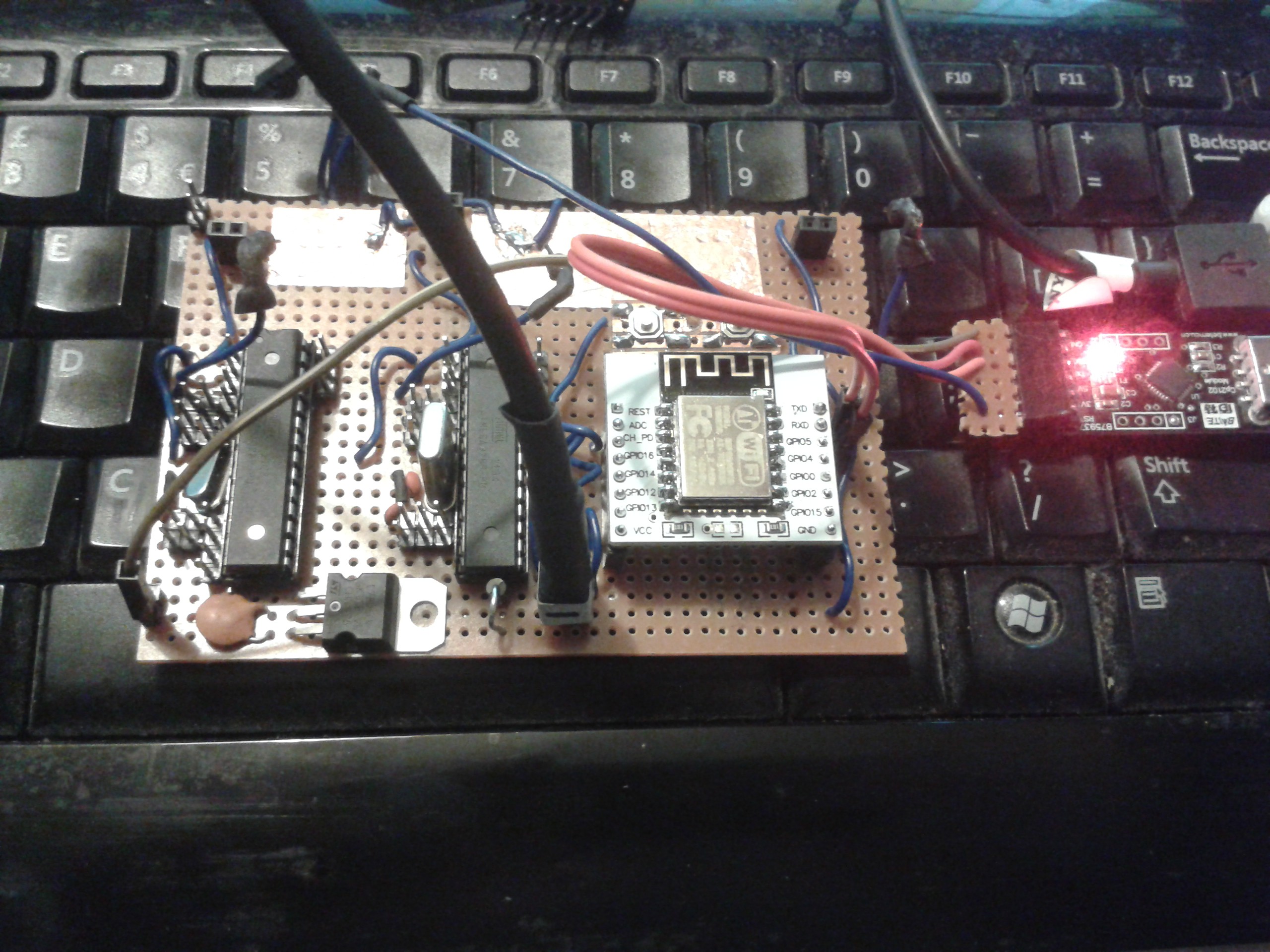
I built this to control the servos...

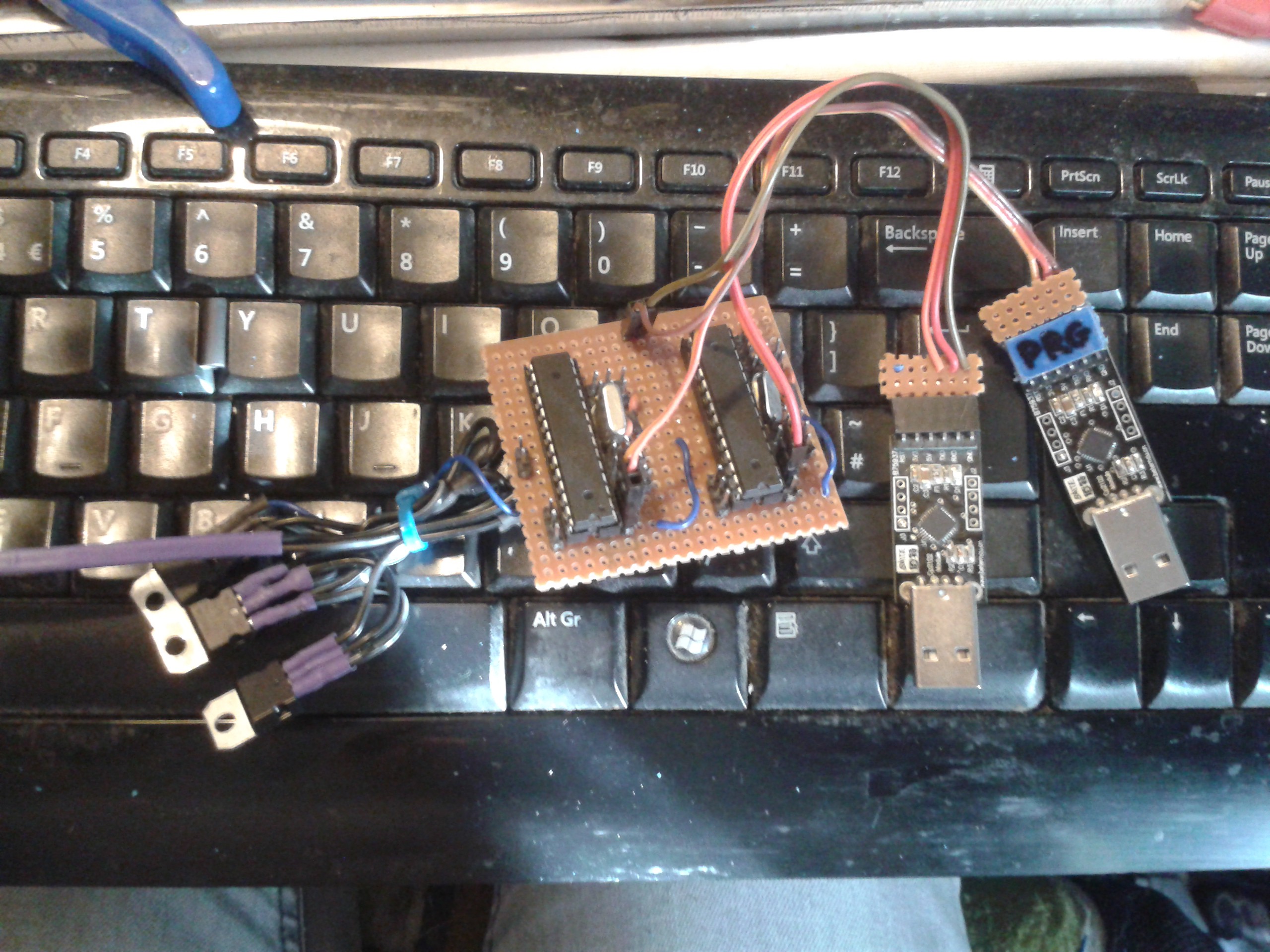
Using the multiprocessor serial networking. The TX of each is on a flylead that plugs into the RX of the next, and its broken out on the top left corner so I can connect the TX and RX of the UART.
Its powered by a 5V 2A supply, and the whole thing is paranoically well grounded and shielded to prevent any crosstalk.

Here the ESP is connected directly to the UART and has been programmed with multicore.ino:

const int host=1;
const int packlen=1;
unsigned char bytes;
int bootdelay;
void setup() {
  Serial.begin(115200);                           // open serial port
  while (!Serial) { ; }                           // wait for the port to be available
  if (host==1) { bootdelay=1000; } else { bootdelay=5000; }
  for (int d=0; d<bootdelay; d++) {               // garbage collect delay
    if (Serial.available() > 0) { unsigned char dummy=Serial.read(); }
    delay(1);
  }
  
} 
void loop() { 
  int val1;
  if (Serial.available() > 0) {                  // if there is a packet
    bytes=Serial.read();                          // read the packet
    val1=(int)bytes;
 
      Serial.write(bytes);                    // write packet
      
  }
}

Which has had everything stripped out so all it does is return what it is sent. It can be uploaded to the ESP and the Atmel without modification and should perform the same. On an Atmel, viewed from a simple port scanner and byte injector script:

Port not open
Clearing buffers...
Connected!
Starting input thread.
Send command byte
Byte : 1
00000001 - 01 - 1  
Send command byte
Byte : 2
00000010 - 02 - 2  
Send command byte
Byte : 3
00000011 - 03 - 3  
Send command byte
Byte : 255
11111111 - ff - 255 - �
Send command byte
Byte : 
Thread done!
Main done!

However, uploaded to an ESP (and I have now tried two, one from eBay and one that Ars sent me) it does this instead.

Send command byte
Byte : 3
00000011 - 03 - 3  
00000000 - 00 - 0  
00000000 - 00 - 0  
11111110 - fe - 254 - �
11111110 - fe - 254 - �
Send command byte
Byte : 3
00000011 - 03 - 3  
Send command byte
Byte : 3
00000011 - 03 - 3  
Send command byte
Byte : 4
10000010 - 82 - 130 - �
Send command byte
Byte : 1
11000000 - c0 - 192 - 
Send command byte
Byte : 1
11000000 - c0 - 192 - 
Send command byte
Byte : 2
00000010 - 02 - 2  
11111111 - ff - 255 - �
00000000 - 00 - 0  
00000000 - 00 - 0  
11111111 - ff - 255 - �
Send command byte
Byte : 00000000 - 00 - 0  
00000000 - 00 - 0  
11111100 - fc - 252 - 
11111110 - fe - 254 - �
11111110 - fe - 254 - �
11110000 - f0 - 240 - 
11111100 - fc - 252 - 
11111111 - ff - 255 - �
11110000 - f0 - 240 - 
11111110 - fe - 254 - �
11111010 - fa - 250 - 
11111111 - ff - 255 - �
11111111 - ff - 255 - �
00000000 - 00 - 0  
11100000 - e0 - 224 - 
10000000 - 80 - 128 - �
11000000 - c0 - 192 - 
11111000 - f8 - 248 - 

Of particular note is the last section. While I was sitting and puzzling over where all the spare bytes were coming from, an few more appeared at random. Then a few more, and more as I watched. Eventually it filled up the terminal over about 10 minutes in random bursts.

The Atmels dont do it using the same code on the same board, same power supply and connected to the same rig, so I really have no explanation other than I have two bad processors and I've wasted my time trying to get something broken to work. Its making up data on its own, no wonder I couldnt get anything meaningful out of perfectly good code - which I wrote blind I might add. Runs on the Atmels without modification, but I had to add garbage collection and checksumming just to get it to run with the ESP and now I know why.

I've built two motherboards, one using brand-new hardware, hacked a test rig with flyleads and Arduinos and a ESP programmer board I built, nothing worked, finally I strip it all back and watch it taking the piss...