Before building the hardware, the design should be simulated. Ideally, we would like to have a spectrometer design covering 400-1000nm, but cleanly covering the full 400–1000 nm needs a more complex (and costly) order-sorting filter, which goes against our aim of an affordable, user-modifiable instrument.  This log covers a cost-optimised design: a budget design for 500–1000 nm built entirely from 1‑inch off‑the‑shelf lenses and a short Hamamatsu linear detector. The challenge: how much performance can you squeeze out of affordable, standard parts?

The optic design uses BeamFour, a free ray‑tracer, plus small Python scripts to derive the spot size. No expensive optics software needed.

We will walk through the design, then explain every parameter we use to judge it, so the charts further down make sense even if you've never touched optics software.

The design

Light comes in from an optical fiber, gets collimated (turned into a parallel beam) and re-imaged 1:1 onto a narrow entrance slit. That slit is the "object" the spectrometer looks at. After the slit, a lens collimates the light again and sends it onto a diffraction grating, which is the part that actually splits broadband light into its colours by bending each wavelength through a slightly different angle. A final camera lens focuses each colour to its own spot on the detector. Because different colours land at different positions, the detector sees the spectrum — a strip of light where position equals wavelength.

It's called a 4f design because the lenses are spaced by their focal lengths in a way that keeps the beam well-behaved, and it's folded (bent with the grating and layout) so the whole thing fits in a small box.

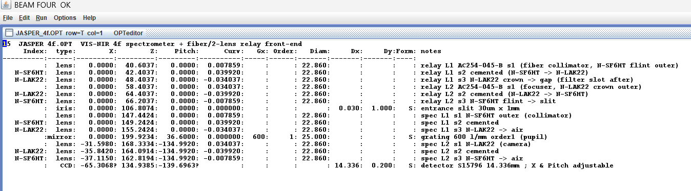
Figure 1: The JASPER 4f prescription in BeamFour. Each row is one optical surface — the four doublets, the 30 µm slit, the 600 l/mm grating, and the tilted S15796 detector.

This is the actual "recipe" for the instrument, as BeamFour stores it. Each line is one optical surface — one face of a lens, the slit, the grating, or the detector — described by where it sits and how strongly it's curved. Reading it top to bottom follows the light:

• Four identical doublets (AC254-045-B). A doublet is a lens made of two glasses cemented together (here a crown glass, N-LAK22, and a flint glass, N-SF6HT). Gluing two glasses together cancels most of the colour smear a single lens would add. All four lenses in the system are the same stock 45 mm, 1-inch Thorlabs part — that's the "cost-optimised" part of the story. Two form the fiber relay, one is the collimator, one is the camera.
• The 30 µm entrance slit. Listed as the iris, 0.030 mm wide.
• The grating, 600 lines per mm, working in first order — the disperser.
• The detector (CCD), a Hamamatsu S15796, 14.336 mm long, whose position and tilt we're allowed to adjust.

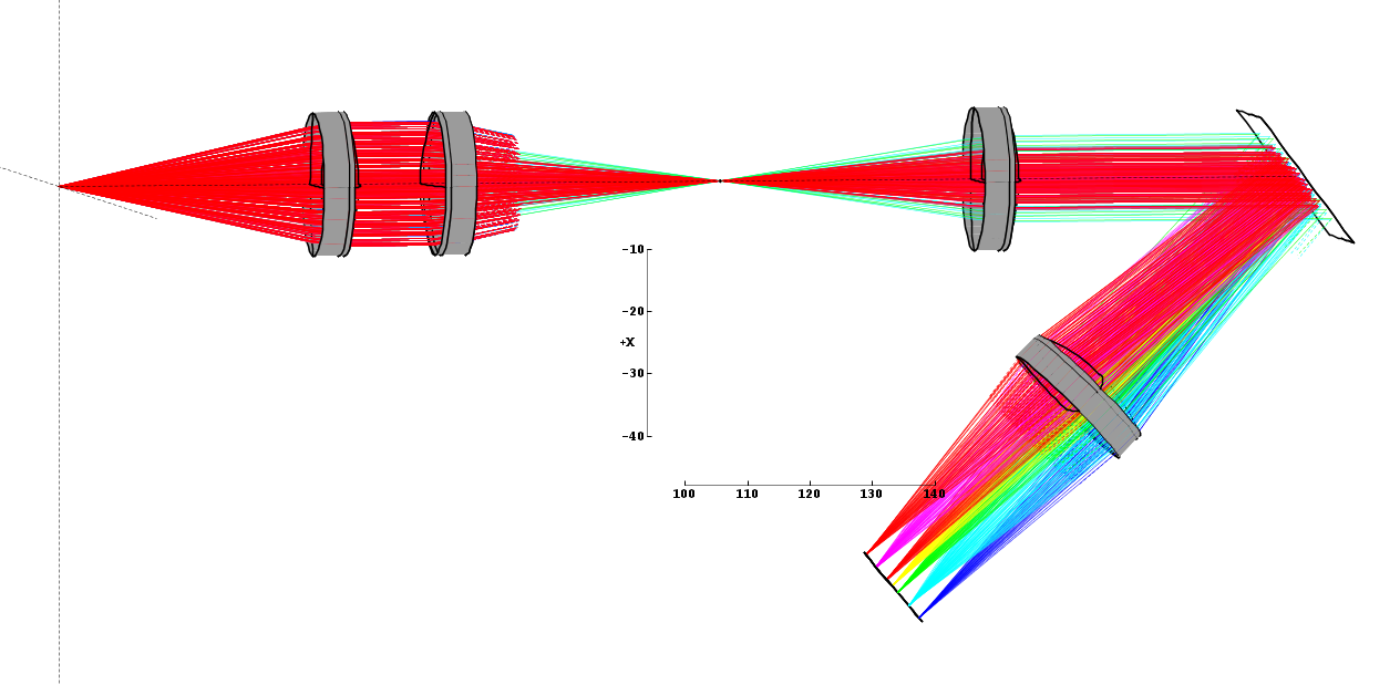
Figure 2: BeamFour ray trace of the full folded path: fiber → 1:1 relay → slit → collimator → grating → camera lens → tilted detector. The colours fanning out at bottom right are the 500–1000 nm spectrum being sorted onto the sensor.

This is what a ray trace looks like: the software fires hundreds of light rays through the design and draws where each one goes. On the left, the fiber light is relayed to the slit (the pinch point in the middle). It's then collimated, hits the grating, and the camera lens (lower right) focuses it down.

The rainbow fan at the bottom right is the whole trick of a spectrometer made visible — the grating has bent each colour by a slightly different angle, so red, green and blue rays arrive at different places on the detector. That spread along the detector is the spectrum.

How we judge the design — the parameters:

Before the analysis charts, here's what each number means. Every one of these is measured from the traced rays.

Spot / spot diagram. When the camera focuses one single colour, it should ideally land as one perfect point. In reality it lands as a small smudge of rays called a spot. A spot diagram is just a zoomed-in picture of where all the rays for one colour actually hit. Smaller, tighter spot = sharper instrument.

Centroid. The average position of all the rays in a spot — i.e. the "middle" of the smudge. For the dispersion direction, the centroid is where that colour's spectral line effectively sits on the detector.

RMSx — the number that sets resolution. RMS stands for root-mean-square, which is just a careful way of saying "typical spread." RMSx measures how far the rays are spread out along the direction colours are separated (the dispersion axis). We only care about this direction, because spreading sideways doesn't blur one colour into the next — only spreading along the colour axis does. In one line: RMSx = √⟨(x − centroid)²⟩, converted to microns. Smaller RMSx = a sharper spectral line.

GEO — the worst-case spot size. Where RMSx describes the typical spread, GEO (geometric radius) is the distance from the centroid to the single farthest ray in the spot. It's the full footprint — the circle that contains every ray. It's always bigger than RMSx and is driven by the most poorly-behaved ray at the edge of the beam. We report it as a reality check on how large the spot can get.

Airy disk / diffraction floor. Physics says no lens can ever focus light to a perfect point — diffraction spreads it into a tiny blob called the Airy disk. Its size is fixed by the wavelength and the lens speed (about 2 µm here). This is the best case: no design can beat it. In our spots it shows as a tiny centre dot. Because our real spots are 10–40× larger than this dot, the design is geometry-limited — meaning lens imperfections, not diffraction, are what set the blur. (BeamFour is a geometric tracer, so it can't model diffraction directly; we draw the Airy disk in as an analytic reference, using the standard formula 1.22 × wavelength × f-number.)

Dispersion scale (nm/mm). How many nanometres of spectrum are packed into one millimetre of detector. Here it's 38–40 nm/mm. Lower would mean the colours are spread out more (finer detail); higher means they're squeezed together. It's not constant across the band, so we always measure it locally from the traced spots rather than using one average.

Spectral span. The total length the whole 500–1000 nm spectrum occupies on the sensor — 13.26 mm here.

Detector fill. What fraction of the sensor's length the spectrum actually uses. 92% means we're filling almost the whole 14.336 mm sensor — good, because unused sensor is wasted resolution.

Δλ (delta-lambda) — the delivered resolution. This is the bottom-line number: the smallest wavelength difference the instrument can actually distinguish, in nanometres. Smaller is better. It's built by combining the three things that blur a spectral line, added in "quadrature" (square them, add, square-root — the right way to combine independent blurs):

Δλ = √( slit-image² + (2.355 × RMSx)² + pixel² ) × dispersion scale

• slit image — the finite width of the slit projected onto the detector (30 µm, slightly narrowed by geometry),
• 2.355 × RMSx — the optical blur. The 2.355 converts the RMS spread into a FWHM (full-width-at-half-maximum), which is the ideal way to state a line width,
• pixel — the detector's 14 µm pixel, which can't resolve anything finer than itself.

rays n / 127 — survivors vs launched. For each colour we launch 127 rays arranged in a pattern across the beam. Some get clipped by the edges of lenses or apertures on the way through (this is called vignetting). The n / 127 count tells you how many survived to reach the detector. A lower number means more of that colour's light is being lost, so its measured spot rests on fewer rays.

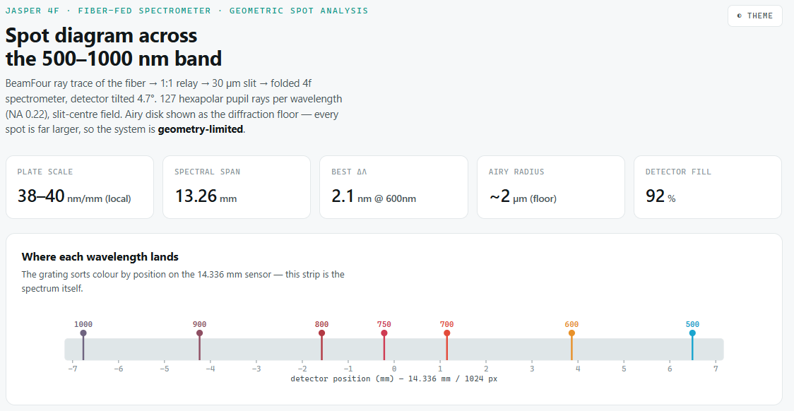
Figure 3: Top-level results. The five tiles summarise the whole design; the strip below shows exactly where each wavelength lands on the 14.336 mm sensor — that strip is the spectrum itself.

The five tiles are the headline numbers, now that you know what they mean: dispersion scale 38–40 nm/mm, the spectrum spanning 13.26 mm, a best-case resolution of 2.1 nm (at 600 nm), the ~2 µm diffraction floor, and 92% of the sensor used.

The strip underneath is the most intuitive picture in the whole analysis: it's the sensor drawn to scale, with a coloured tick showing where each wavelength actually focuses. This is, quite literally, the spectrum the instrument would produce.

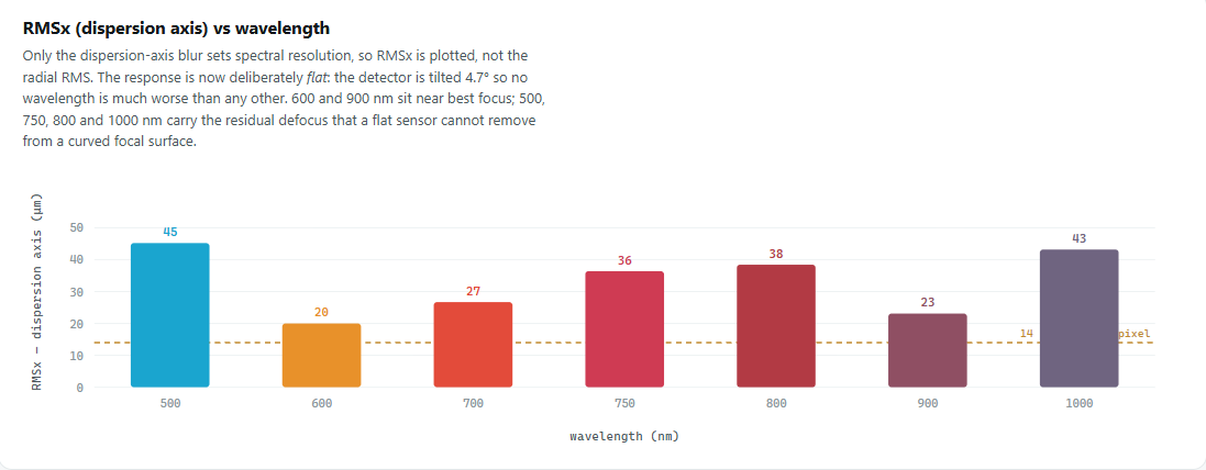
Figure 4: RMSx (spectral-axis blur) for each wavelength. The dashed line is one detector pixel. The response is deliberately flat — no wavelength is far worse than the others.

This bar chart shows RMSx at each wavelength. The interesting thing isn't any single bar — it's that they're all roughly similar height. That flatness is on purpose. 600 and 900 nm sit near best focus (sharpest); 500, 750, 800 and 1000 nm carry a bit of leftover blur. But nothing is catastrophically bad, which is exactly what you want in a spectrometer that has to work across the whole band, not just in the middle.

The dashed line marks one 14 µm pixel, so you can see the blur in units of "how many pixels wide is this."

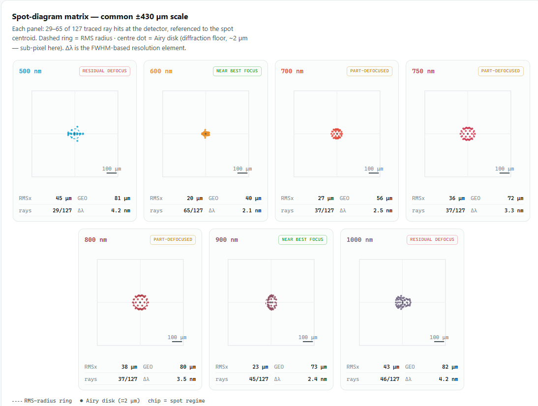
Figure 5: One spot per wavelength, all drawn to the same ±430 µm scale. Dashed ring = RMS radius, centre dot = the ~2 µm Airy disk. The small print under each panel gives RMSx, GEO, the surviving ray count, and Δλ.

Now you can read every panel. Each shows the actual cloud of surviving rays for one colour, all on the same scale so they're comparable. The tiny centre dot is the diffraction floor (the best any optics could do); the fact that every real spot dwarfs it is the visual proof that we're geometry-limited. Under each panel are the four numbers we defined: RMSx, GEO, rays-survived, and Δλ.

Notice the shapes differ — some are tight blobs, some are little rings or arcs. Those shapes are the fingerprints of specific lens aberrations, which leads to the one genuinely surprising result.

The surprise: it's not the colours, it's the curved focus

The obvious guess for why the band edges (500 and 1000 nm) are softer than the middle is chromatic aberration — the classic problem where a lens focuses different colours at slightly different distances. It's the intuitive villain.

But when we isolated the camera lens and tested it two ways, the data said otherwise:

• Hold the colour fixed and only change the angle the light enters at (which is what really changes as you move across the band): best focus moved by about 2.3 mm. This is field curvature — the lens focuses onto a gently curved bowl-shaped surface, not a flat plane, so off-centre colours focus at a slightly different depth.
• Hold the angle fixed and sweep the colour across the whole 500–1000 nm range: best focus moved only about 0.37 mm. That's the actual chromatic effect — and it's tiny.

So the real limiter is field curvature, about six times bigger than the colour effect. The doublets are doing their job on colour; it's the flat sensor trying to catch a curved focus that costs us sharpness.

That's also why the detector is tilted 4.7°. A tilt can't un-bend a curved focal surface, but it can line the sensor up as well as possible with it — trading a little sharpness in the middle to rescue the ends. It's why the RMSx chart is flat rather than pointy.

The ceiling

There's a hard limit hiding in the geometry. Squeezing 500 nm of spectrum onto a 14.336 mm sensor forces about 37–40 nm/mm, and once you fold in the pixel size, the finest resolution this sensor can ever deliver is around 1 nm — no matter how perfect the glass is. We're already within about 3× of that wall.

So the biggest single upgrade isn't fancier lenses — it's a longer detector. A 29.1 mm sensor would roughly halve the dispersion scale and unlock the resolution the optics are capable of. That's the next move.

Why this approach

The whole point of doing this in BeamFour plus Python — rather than a costly commercial tool — is that it's reproducible and free. We even wrote a small Python tracer that reproduces BeamFour's output exactly, so we can scan hundreds of "what if we tilt the detector 0.1° more?" variations offline in seconds, then confirm the winner with a real BeamFour trace. BeamFour stays the authority; Python just makes the search fast.

If you're building a spectrometer on a budget, the takeaway is that stock 1-inch doublets and a free ray tracer get you to a genuinely useful VIS–NIR instrument — and that reading the spots carefully tells you exactly which part to spend your next rupee/dollar on. For us, that's the detector, not the lenses.

Quick glossary

• Spot — the little smudge of rays one colour actually focuses to (ideally a point).
• Centroid — the average/centre position of a spot.
• RMSx — typical spread of the spot along the colour axis; sets resolution. Smaller = sharper.
• GEO — distance to the farthest ray; the worst-case spot size.
• Airy disk — the ~2 µm diffraction limit; the smallest spot physics allows.
• Geometry-limited — spots are far bigger than the Airy disk, so lens shape (not diffraction) sets the blur.
• Plate scale — nanometres of spectrum per millimetre of detector (38–40 nm/mm here).
• Spectral span — how long the full spectrum is on the sensor (13.26 mm).
• Detector fill — fraction of the sensor used (92%).
• Δλ — the delivered resolution: smallest wavelength gap the instrument can separate.
• FWHM — full-width-at-half-maximum, the honest width of a blurred line (= 2.355 × RMS).
• Vignetting — rays clipped by lens/aperture edges; why not all 127 launched rays survive.
• Field curvature — the lens focuses onto a curved bowl, not a flat plane — our real limiter.
• 4f / folded — a compact lens spacing, bent to fit in a small enclosure.