Right now my Lunar Lander looks a lot like Spacewar! and Computer Space, a ship flying around in the blackness of space. What makes Lunar Lander unique is the moonscape at the bottom of that screen. One might say that Lunar Lander is more grounded as a result.

I use the term "moonscape" loosely. In the original, the ground is just a 2D low detail representation of some hilly terrain drawn using vector graphics as a single solid line. Never the less the way that line smoothly transitions as it changes direction "feels" like the land it represents.

On the PDP-1, I do not have the pixel "budget" to draw a curvy solid line from the left to the right side of the screen. That would be over a thousand pixels. At most the PDP-1 is only capable of refreshing a few hundred pixels each frame. Since the terrain is an important part of the game I think a hundred pixels is a reasonable allocation for drawing it.

So generate some "realistic" looking terrain using only a hundred pixels. No Problem. 

Actually it turns out there is a LOT of information on generating 2D and 3D terrain, mostly coming out of the gaming community.  There are a number of techniques for taking some height samples and smoothing them into something that mimics "land" to the eye. One of these is cosine interpolation.  

Cosine interpolation is a smooth, curved method for estimating values between two points, using a portion of a cosine wave to create a natural-looking transition. It is often used to generate more aesthetically pleasing curves for periodic or oscillating data.

I was lucky enough to find a Python script that was exactly tailored to my needs. I spent considerable time trying to re-locate the source so that I could credit them, but was unsuccessful. So to the author: Thank you so much.

import numpy as np
import matplotlib.pyplot as plt

def cosine_interpolation(y1, y2, mu):
    """
    Performs cosine interpolation between two points.
    
    Args:
        y1 (float): The value of the first point.
        y2 (float): The value of the second point.
        mu (float): The interpolation factor (0.0 to 1.0) indicating the
                    relative distance between the points.
                    
    Returns:
        float: The interpolated value.
    """
    mu2 = (1 - np.cos(mu * np.pi)) / 2
    return y1 * (1 - mu2) + y2 * mu2

def smooth_terrain_with_cosine(data, num_new_points):
    """
    Smooths 1D terrain data by interpolating new points between existing ones
    using cosine interpolation.

    Args:
        data (np.array): The original 1D terrain data.
        num_new_points (int): The total number of points desired in the smoothed data.

    Returns:
        np.array: The new, smoothed terrain data.
    """
    # Original data points indices
    x_old = np.linspace(0, 1, len(data))
    
    # New points indices
    x_new = np.linspace(0, 1, num_new_points)
    y_new = np.zeros(num_new_points)
    
    # Calculate the number of original data points
    n_original = len(data)

    for i, x_val in enumerate(x_new):
        # Find the two nearest original data points
        # np.searchsorted finds the index where x_val would be inserted to maintain order
        idx_right = np.searchsorted(x_old, x_val, side='right')
        
        # Handle boundary cases for the last point
        if idx_right == n_original:
            y_new[i] = data[-1]
            continue
            
        idx_left = idx_right - 1

        # Get the y values of the surrounding points
        y1 = data[idx_left]
        y2 = data[idx_right]
        x1 = x_old[idx_left]
        x2 = x_old[idx_right]
        
        # Calculate the interpolation factor (mu)
        mu = (x_val - x1) / (x2 - x1)
        
        # Perform cosine interpolation
        y_new[i] = cosine_interpolation(y1, y2, mu)
        
    return y_new

# --- Example Usage ---

# 1. Generate some sample terrain data (e.g., random heights at fixed intervals)
original_data = [400, 240, 240, 100, 30, 30, 70, 70, 40, 40, 40, 40, 80, 120, 160, 160, 240, 320, 360,360]

# 2. Define the desired total number of points for the smoothed terrain
smoothed_points_count = 100

# 3. Smooth the data
smoothed_data = smooth_terrain_with_cosine(original_data, smoothed_points_count)
#print(smoothed_data)

# 4. Plot the results
plt.figure(figsize=(10, 6))
plt.plot(np.linspace(0, 1, smoothed_points_count), smoothed_data, label='Cosine Smoothed Terrain', color='blue')
plt.scatter(np.linspace(0, 1, len(original_data)), original_data, color='red', zorder=5, label='Original Data Points')
plt.title('1D Terrain Smoothing using Cosine Interpolation')
plt.xlabel('Normalized Distance')
plt.ylabel('Height')
plt.legend()
plt.grid(True, linestyle='--', alpha=0.6)
plt.show()

# 5. Convert the data into x,y coordinates that lunar lander can use.
#    Coordinates will be put into 18 bits with x occupying the upper
#    9 bits and y the lower nine bits.
x = 0
count = 0
for y in smoothed_data:
    # Convert the coordinates to PDP-1 screen space.
    sx = x - 511
    if sx < 0:
        sx = abs(sx) ^ 0b1111111111
    sy = int(y) - 511
    if sy < 0:
        sy = abs(sy) ^ 0b1111111111
        
    # Drop the least significant bit of each coordinate and pack into 18 bits.
    xy = ((sx>>1)<<9)+(sy>>1)
    print(count, str(x-511).zfill(3),str(int(y)-511).zfill(3),bin(sx),bin(sy),bin(xy)[2:].zfill(18),'\t\t',oct(xy)[2:].zfill(6))
    x = x + 10
    count = count + 1
    
print("y-coordinates")
count = 0
for y in smoothed_data:
    print(count,str(int(y)).zfill(3),'\t\t',oct(int(y))[2:].zfill(6))
    count = count+1

 All I had to do was:

• Add my terrain data in original_data. I entered 20 height values into the array that defined the general shape that I wanted the "ground" to be.
• Set smoothed_points_count to be 100, the number of points I wanted.
• Add code (#5) to take the generated data and convert the points to screen coordinates in a format that would be efficient to plot. I borrowed this idea from ICSS where coordinates are put into an 18 bit word with x occupying the upper 9 bits and y the lower nine bits and the least significant bit assumed to be 0.

That's it. When I ran the script it emitted a plot of what it had done.

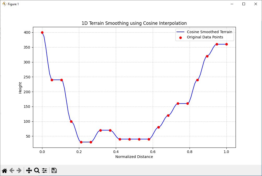
It's elongated in the vertical direction but totally what I was looking for. Then here are my 100 terrain points in octal format ready to drop into the lunar lander code.

trn,    400710
        405700
        412656
        417626
        424602
        431570
        436570
        443570
        450570
        455570
        462570
        467565
        474551
        501525
        506501
        513464
        520461
        525454
        532442
        537430
        544421
        551416
        556417
        563417
        570417
        575417
        602417
        607420
        614425
        621433
        626440
        633442
        640443
        645443
        652443
        657443
        664443
        671442
        676440
        703433
        710427
        715424
        722424
        727423
        734424
        741424
        746424
        753424
        760424
        765424
        772424
        777424
        004424
        011424
        016424
        023424
        030424
        035424
        042424
        047430
        054436
        061444
        066447
        073450
        100453
        105461
        112467
        117473
        124474
        131476
        136503
        143511
        150516
        155517
        162520
        167520
        174520
        201520
        206520
        213522
        220533
        225546
        232561
        237567
        244571
        251600
        256614
        263627
        270636
        275640
        302643
        307650
        314656
        321662
        326664
        333663
        340664
        345664
        352664
        357664

And finally I added the code to plot the terrain.

/ Draw the terrain.
        init dti, trn         / Point to first word of terrain data.
        jsp dtr               / Draw the terrain.
...

dtx,    jmp .
dtr,    dap dtx
dti,    lac .                 / Get the next terrain data word.
        sza i                 / Is 0?
        jmp dtx               /  Yes - return.
        cli                   / Set the y coordinate.
        scr 9s                / Shift low 9-bits into the high 9-bits of IO.
        sal 9s                / Move remaining 9-bits into the high part of AC.
        dpy-i 4300            / Plot the point.
        idx dti               / Bump the data address to the next point.
        jmp dti               / Continue.

And with that my blogging has caught up with where I actually am in program development. Here is the What I Have So Far video again.