Joan Horvath
-
Log #9: Example - PID controller
08/16/2017 at 01:35 • 0 commentsApplying these ideas: a PID controller
At the beginning of our project, we talk about calculus as being useful to understand how things move and change. Often we want to control how things move and change in a predictable way. One extremely common way of doing that is with a PID controller, which stands for “proportional-integral-derivative.”
Historically these were analog devices, and now are algorithms, that attempt to control something to a set value by using a mix of the current value, its integral (the sum of its value for some period in the past, effectively a smoothed past value) and its derivative (how fast, and in what direction, it is changing).
PID controllers are often correcting for some type of systematic error – friction, cooling, etc. They take data on some regular interval (“sampling”) and use how much that signal differs from a desired set value (the “error”) to send an adjustment to whatever it is they are measuring. For example, if something was trying to hold a temperature at 200 degrees and it measured 199 one sample ago and 201 now, the error one time step in the past would be -1 and now would be 1.
However, it’s a little trickier than that. There is a finite delay as the signal propagates through the system from the controller’s output back to its input. Let’s say that this delay is 3 time samples, for the sake of illustration. Then the inputs to calculate the next error signal that the controller will use are taken at the array of times shown in the picture.
 Graph showing which time steps are used for each algorithm
The derivative term allows the controller to react to short-term errors that take the system too far away from its set point. The integral balances that out by essentially tracking any long-term systematic bias in the system, and correcting for it. If the terms are out of whack, a system might oscillate around or go unstable.
To write is as a sort-of equation:
Error (now, time=0) =
Error at the previous time sample (time = -1)+ Kp * the error back one delay time ago (time = -delay)
+ Ki * Integral of the error, based on a time range from the current time minus the delay back to as far back as the design accumulates (time = - delay back to whenever the controller turned on
+ Kd * Derivative, based on the signal value at times –delay and (–delay-1)
+ a modeled systematic outside error (a steady drift, sinusoidal noise, etc.)
Kp, Ki, and Kd are constants that can be created semi-empirically or based on a model of the system being controlled evaluated at time step -1.
PID controllers are everywhere, and have been around in some form or another for hundreds of years (for a history, see https://en.wikipedia.org/wiki/PID_controller.) Christian Huygens created a mechanical predecessor around the same time that Newton was working on calculus -- a “centrifugal governor” to manage how much grain was milled by a windmill as the windspeed changed. Nicholas Minorsky is credited with being the first person to write down the relevant math in 1922.
Numerical derivatives and integrals
We thought it would be interesting to find a way to model and view a simulated PID controller. In our integral and derivative models so far, we’ve just used the equations for a curve and its integral and derivative, which we figured out the traditional algebraic way. However, here, we do not have an actual function, so we need to integrate and differentiate in a discrete way. We could have done our curve-and-its-differential/integral models that way too, and we will probably create a generalized version there too.
At any rate, there are a lot of ways to do discrete derivatives (more usually called “finite differences”) and integrals. For now, we are using the most simple-minded way. That is, for a derivative of a curve we use the difference of the values of the curve at the most recent two time points. We should be dividing by the time step between when these were taken, but we since we are scaling everything by arbitrary scaling factors anyway we will assume the time between samples
For the integral, we recursively add on the value of the most recent time step to the sum thus far of all time steps.
There are other formulas that use more time steps or other corrections, but we will worry about those things later. A lot of calculus is festooned with special cases and ways to deal with the fact that not everything works all the time. We think that delving into that too soon is what makes “normal” calculus classes impenetrable. (As an aside for calculus teachers reading this, consider having your students consider the errors and failure modes of these (over) simplified lookback strategies.)
PID model
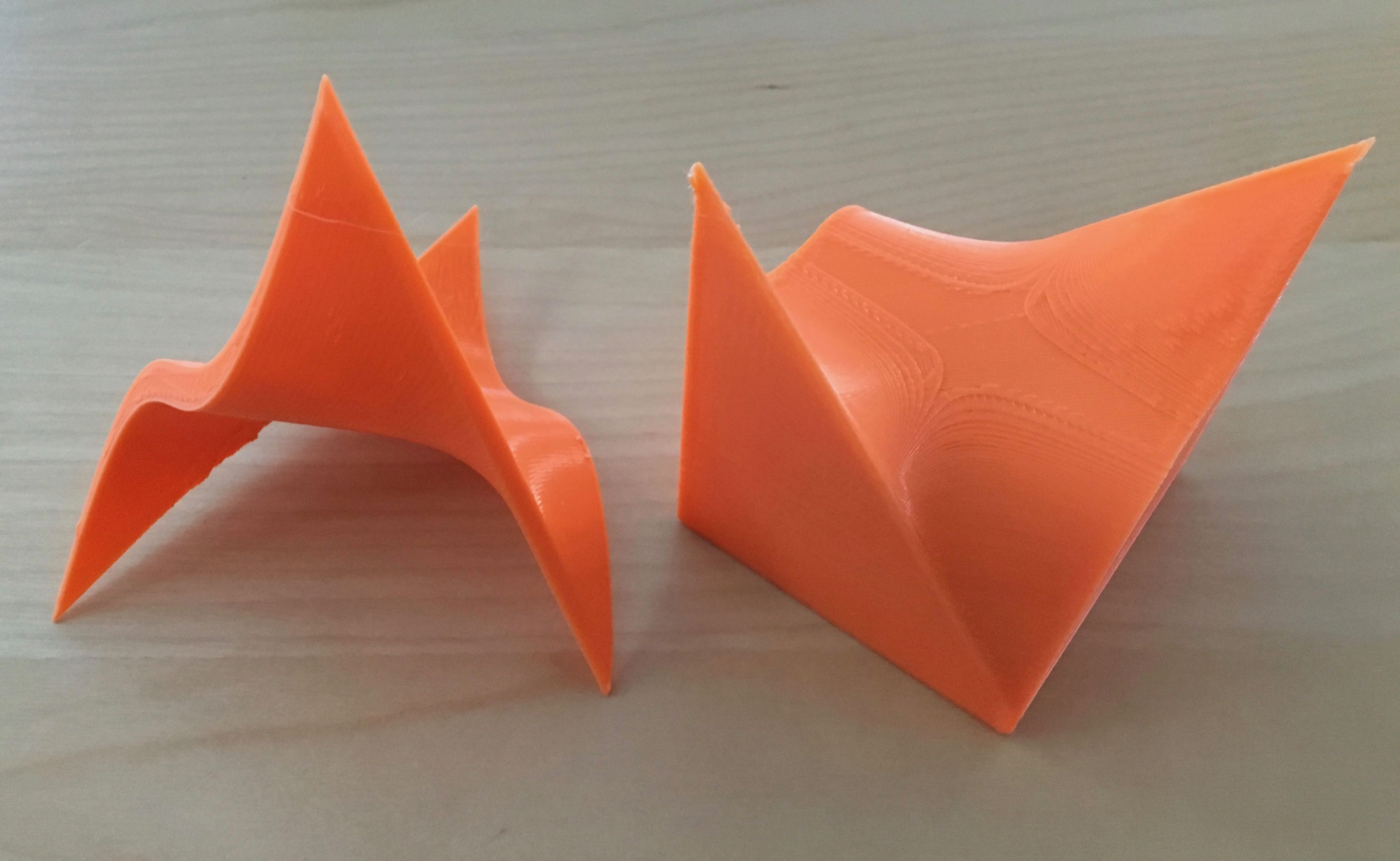
We have created two different PID controller models, and are printing side-by-side the time values of an input noise signal, the error (correction) signal, and the three P-I-D terms (the proportional term, the integral term, and the derivative term).
We designed one to go quickly to the desired steady state, and another to be somewhat unstable.
In the photos, time goes from left to right. Closest to you is the simulated system bias (a constant drift plus a small sinusoidal offset). Next is the error signal we are calculating from summing all these inputs; then the same function time shifted one delay time; then the integral and the derivative. They are all multiplied by scaling factors to be visible; in reality, some of these inputs would be very small.
 PID controller terms graph for stable system
 PID controller terms graph, unstable system
Obviously, you could also graph these curves and look at them all as colored lines on a 2d graph. But we find the third dimension adds some insight and interest.
This is one very specific example of an equation involving a mix of integrals, derivatives and other terms. There are many of these that govern important phenomena. We want to see if there are ways to make combining terms more intuitive, or predicting types of solutions. Currently math students learn a large “toolbox” of these equations and what to do with them, but maybe we can take a more physical approach.
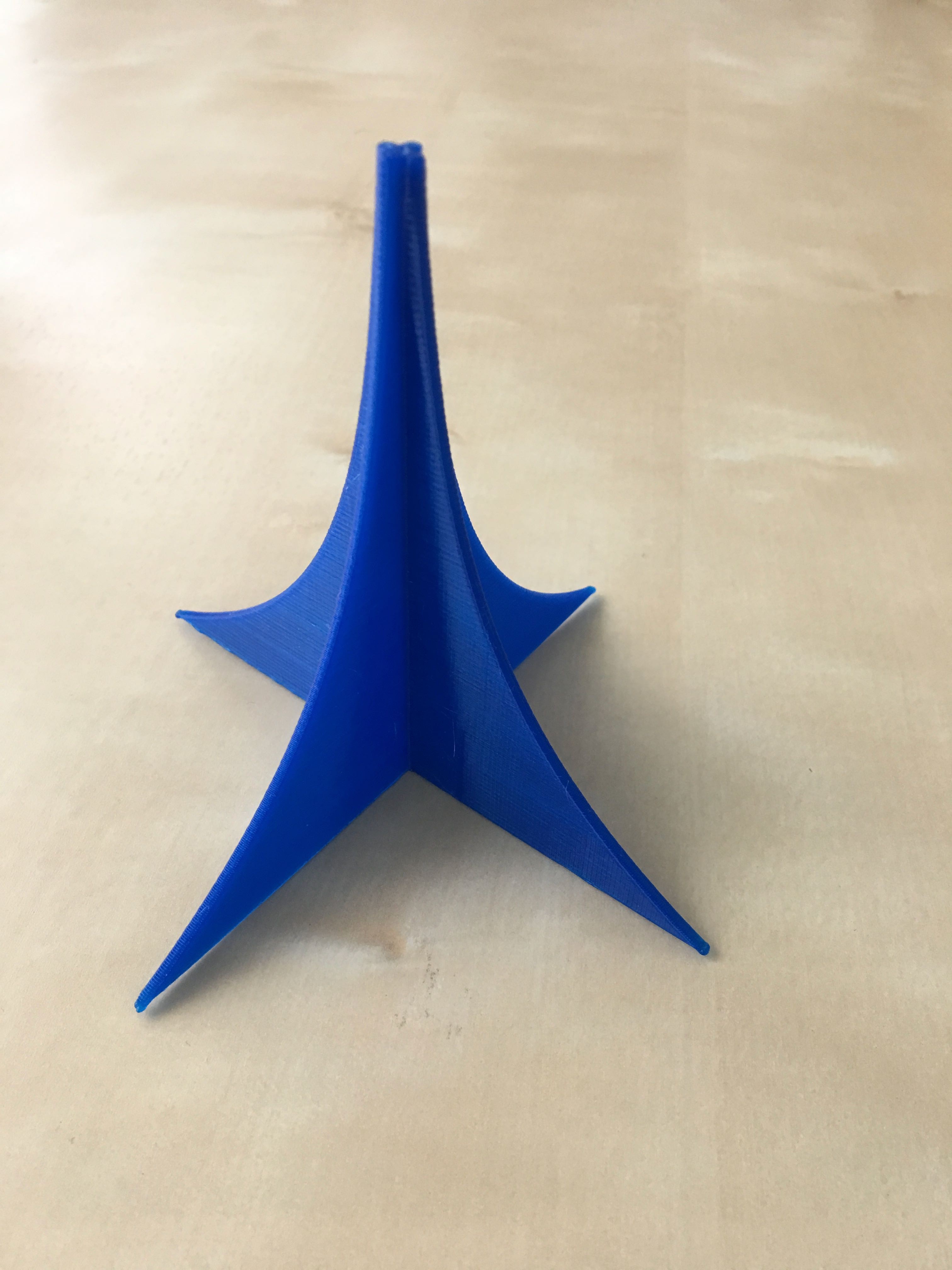
The 3D printable STL files will be included in the FILES section of this project. These were generated in OpenSCAD. These are very much a work in progress and we are thinking about better methods for various aspects of this. But at least you can create and think about these particular ones if you’d like.
A final note: printing the second file was a challenge. It was printed as shown, and we used a cooling tower in the end to get the points to print correctly. See the photo below of the layout on a Bukito. A cooling tower is just a cylinder that is a little taller than a delicate point on a print. It keeps the printer from trying to lay up plastic faster than it can cool and minimizes gloppy points on a print. Note that we scaled the print down by 50% from the size is is in the STL.
 PID print with a cooling tower
 -
Log #8: Interlude - Community Feedback
08/15/2017 at 21:10 • 3 commentsAs we have gone along we have tried to get feedback from various constituencies: people who never took calculus but are curious, people who teach it, people who teach less-advanced math but are interested in adding in these concepts earlier, and so on.
The first advice we got from people focused on the teaching aspect was that it would be too hard to support electronics, 3D printing, and other hands-on activities all in the service of a calculus class. The suggestion was to focus on just one thing and to be sure that the ideas made sense even if someone were just reading about the objects and seeing them in photographs. Otherwise we need to explain each technology used before getting into the calculus part, which admittedly can be a distraction. Our original approach, though (of making things a variety of ways) may still be a valid way to go for schools with an extensive makerspace, and we haven’t completely given up on that.
We were grateful that Yue-Ting Siu, Assistant Professor in the Graduate College of Education at San Francisco State, took a look at some of our early models. Dr. Siu is interested in how best to teach the visually impaired. Obviously 3D prints work best for this constituency (compared to building electronics), and her suggestion was to thing about how to add gridlines and other orienting material to these plots. We are thinking about the best ways to do that within the resolution and surface finish limitations of a 3D printer, and without cluttering the models or making them confusing.
Dr. Siu also suggested that we think about neurodiversity generally and consider how our approach might help other learners who are not served well by traditional education, beyond the visually impaired. As we note in the summary in the "Details" section, we are very interested in exploring this area further with others who have specific expertise.
-
Log #7: The Chain Rule
06/09/2017 at 01:02 • 0 commentsWe discovered that people were quite intrigued by our Fundamental Theorem models (Log #5) and decided we would make some more. We're going to be taking these to some events during the summer and getting more feedback, too.
For now, we are just figuring out what a curve's derivative function is by calculating it using the algebra techniques taught in standard calculus, and then printing out the curve and its derivative at right angles to each other. But we're trying to figure out some good ways to derive some of these geometrically, too.
What happens when you want to take the derivative of something more complicated than a function you can look up in a table of derivatives? The "chain rule" It more or less lets you break down a complicated function into a series of simpler ones.
We will use ^ in what follows to show raising something to a power.
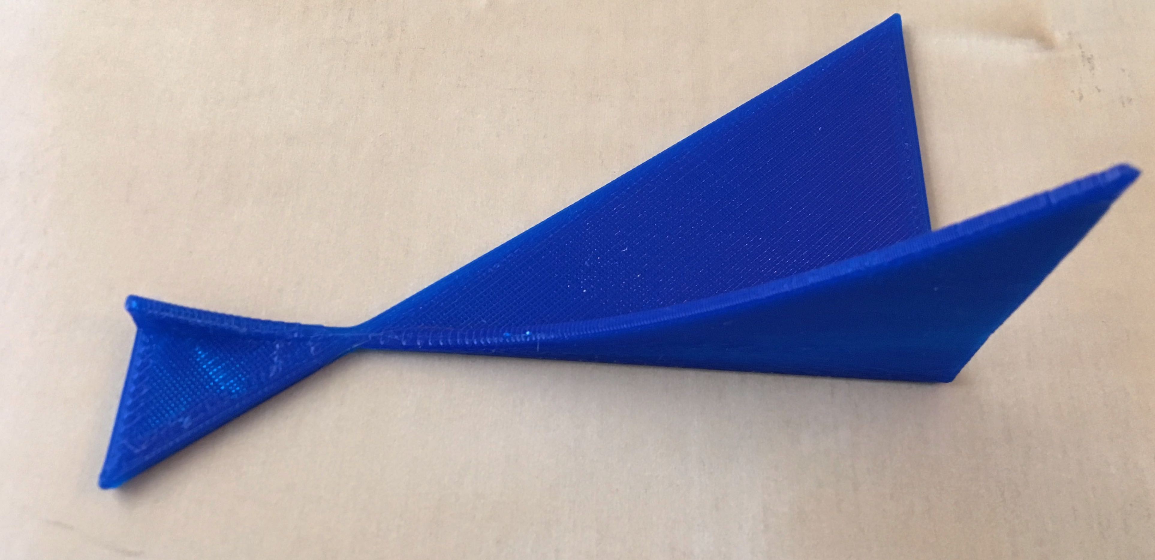
Suppose we want to get the derivative of (sin(x) )^2 - that is, sin(x) * sin(x). Here's what it looks like: the function is the part that is vertical in the picture, and the derivative is the function pointing toward and away from you flat on the table. Or if you prefer the function is the part flat on the table, and its integral is the part sticking up from the table.
![Graph of sin(x) squared and its derivative, sin(x)cos(x)]()
What the chain rule says is:
- First figure out how the function is changing based on how a module of it is changing - here, let's say sin(x) - with respect to that module.
- Then,figure out how that module (here, sin(x)) changes with x.
- Multiply those two pieces together to get the change of the function overall.
Let's do an example, finding the derivative of (sin(x))^2, that is, (sin(x)*sin(x)).
- We can look up that the derivative of x^2 with respect to x is 2x.
- So the derivative of (sin(x))^2 with respect to sin(x) is 2*sin(x).
- Now for the second step we need the derivative of sin(x) with respect to x, since so far we've just figured out how our function changes with respect to sin(x). That is cos(x) -- again, we can look these things up in tables online or in books.
- Finally multiply. The derivative of sin(x) squared = 2*sin(x)*cos(x), which we show in the picture above.
We are thinking about a good way to show the steps of this process physically. Stay tuned! We've found that the chain rule inis credited to Leibnitz. Newton and Leibnitz created calculus at the same time, more or less, and fought over credit as long as Leibnitz was alive (Newton outlived him by quite a bit.)
Newton developed the concepts geometrically, but Leibnitz came up with ways to use algebra to be able to do a lot of things faster. We think though that people can learn it in the first place better with geometrical reasoning. Can we reverse-engineer Leibnitz ideas to make them into geometry? That's our next project- wish us luck!
More Curve-Derivative ( or Integral-Curve) pairs
Meanwhile, we also did a few more pairs so we could more to play with and think about.
Curve x^3 (laying flat on the table) and its derivative 3*x^2 (note, though, that because it was hard to see the shapes of the curves, we have scaled the two curves differently from each other to show the general shapes of the curves).
![Graph of x cubed and its derivative, x squared]()
And here is the curve of ln(x) (facing you) and its derivative, 1/x.
![Curve of ln(x) in foreground, and its derivative 1/x (at right angles)]()
We have had to take some care with scaling and where to start some of these curves. Obviously 1/x can't get too close to x=0, for example. And we've had a lot of experiments where we pushed it a bit too much. Here's an earlier example of the ln(x) and 1/x print. It was a little interesting to get this one off the platform. (Surface on the left was the bottom of the print.)
![]()
We've been really pleased by all the energy we've seen around this idea, and we're working hard to figure out how much geometry-oriented material is needed to really jump-start someone into calculus, and whether some things (like the chain rule) should stay in algebraic form. Lots to think about!
-
Log #6: Sources
05/16/2017 at 20:04 • 0 commentsWe've been asked quite a bit about places to read more. We've gathered all of the interesting ones so far into one web page on our site, so that we can update it easily. Check it out at:
-
Log #5: The Fundamental Theorem in 3D!
05/16/2017 at 03:26 • 0 commentsSo far, we saw that derivatives measure the slope of a curve and tell us how fast things are changing along that curve. We also saw that an integral is just the area under a curve. One of Newton's big insights was that taking the derivative of a curve and finding the integral are what a mathematician would call an inverse operation- they undo each other, just like addition and subtraction. (Purists will note some details here where that is not quite true, but we will get to that later. There is a constant floating around we will need to deal with.)
This insight goes by the grand name of The Fundamental Theorem Of Calculus. We spent some time thinking about how to show this in a hands-on way. We decided to do some specific examples.
![3D graph of straight line and parabola]()
So if I started with a derivative, and integrated it, I would get back the original curve.
If I started with an integral function and took its derivative, I would get back the original curve.
We can look up in tables of integrals and derivatives (we will walk through some common examples in a later log) that the integral of a straight line is a parabola. Or to put it another way, the area under a straight line builds up in a way that turns out to be a parabola. The picture above shows this.
Or, the slope (derivative) of a parabola is a straight line - the slope is negative when the parabola is headed downward to its minimum, and is positive when it is headed up.
Thus, the 3D model above shows a curve and its integral, or a curve and its derivative, depending on which way you want to think about it. This curve could be printed flat, more or less like it is lying on the table here.
Here is an animation (also done in OpenSCAD) of the integral of the area under the line building up as a parabola.
![animation of the integral under a line building up as a parabola]()
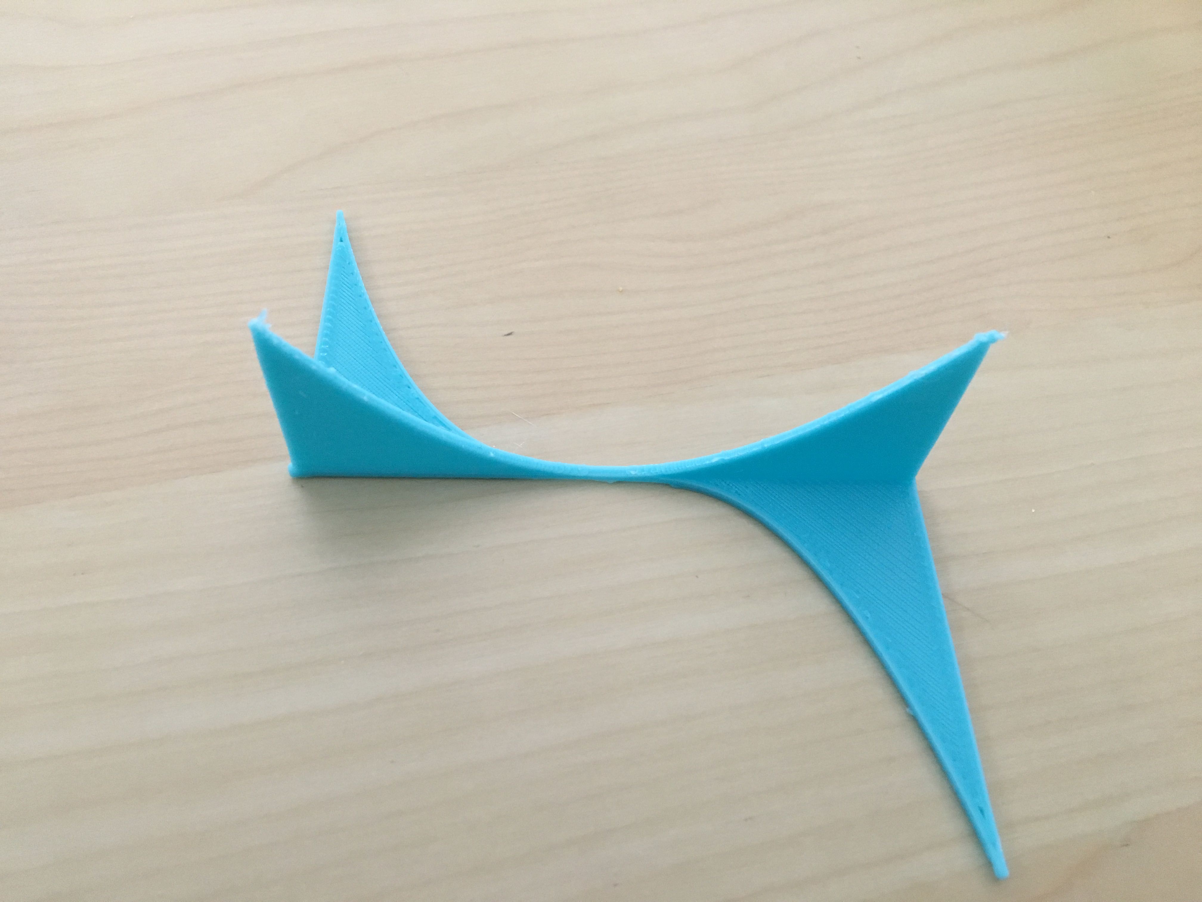
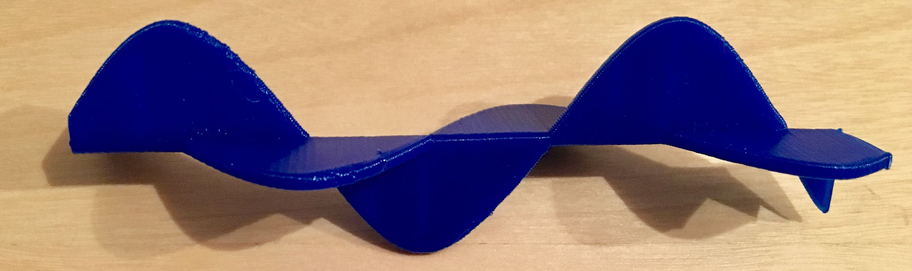
Next, here is a sinusoidal case to think about. Sines and cosines are special in that their derivatives and integrals are other sinusoids, with some fussing around with the signs.
![]()
If we think of the vertical curve as the original curve (say, a sine wave starting at 45 degrees) then the slope is the cosine wave shown in the horizontal curve.
If we think of the horizontal (cosine) curve as the original curve, the vertical curve is its integral (sine). With sines and cosines, the signs flip with the integral so we have to be careful about orientation. Here's the animation:
![Sine and cosine waves, showing how one is the integral of the other]()
We printed the sine and cosine waves here with the same amplitude, but if we were plotting sin(a*x), the derivative would be a*cos(ax), and the integral would be (-1/a) * cos (ax). To make it printable, we ignored this scaling (or you can think of it that we plotted the derivative and integrals with respect to a scaled and offset value.) This print was created vertically, with the side of the model on the left side of this picture on the platform. We used a brim to hold it down.
Lastly, we decided to print a special function, the exponential. The function takes the number e (2.71...) and raises it to the power x, which we can write as e^x. Exponentials have the property that their integrals and derivatives are also exponentials, with some scaling factors thrown in for some cases. We decided to print that as four copies of the exponential- if you keep turning it , you can keep integrating or taking the derivative. It just repeats! (x =0 is at the top of the picture.)
![Exponential function - four copies, one on each axis (sort of looks like a rotor.)]()
All these prints were created with a small OpenSCAD model which takes two functions and plots them at right angles to each other (with a bit of modification for the last model.) We will post this after we do a little cleanup.
We have included two STLs for the fundamental theorem in "Files"- one for the sinusoids here (print vertically with a raft or brim for best results) and another for the squared/cubed pair (photo in log #7) , probably best printed by rotating it for max surface area contact with the platform.)
-
Log #4: Integrals: the Other Half of Calculus
05/04/2017 at 05:50 • 1 commentWe have been talking about differential calculus- the study of how something is changing. There’s another half, though – called integral calculus. Loosely speaking, integral calculus is the process of reversing what you do with differential calculus. You can start with a derivative, and figure out what the original curve was. Think of it like addition and subtraction being inverses of each other. It’s just a little bit more complicated here.
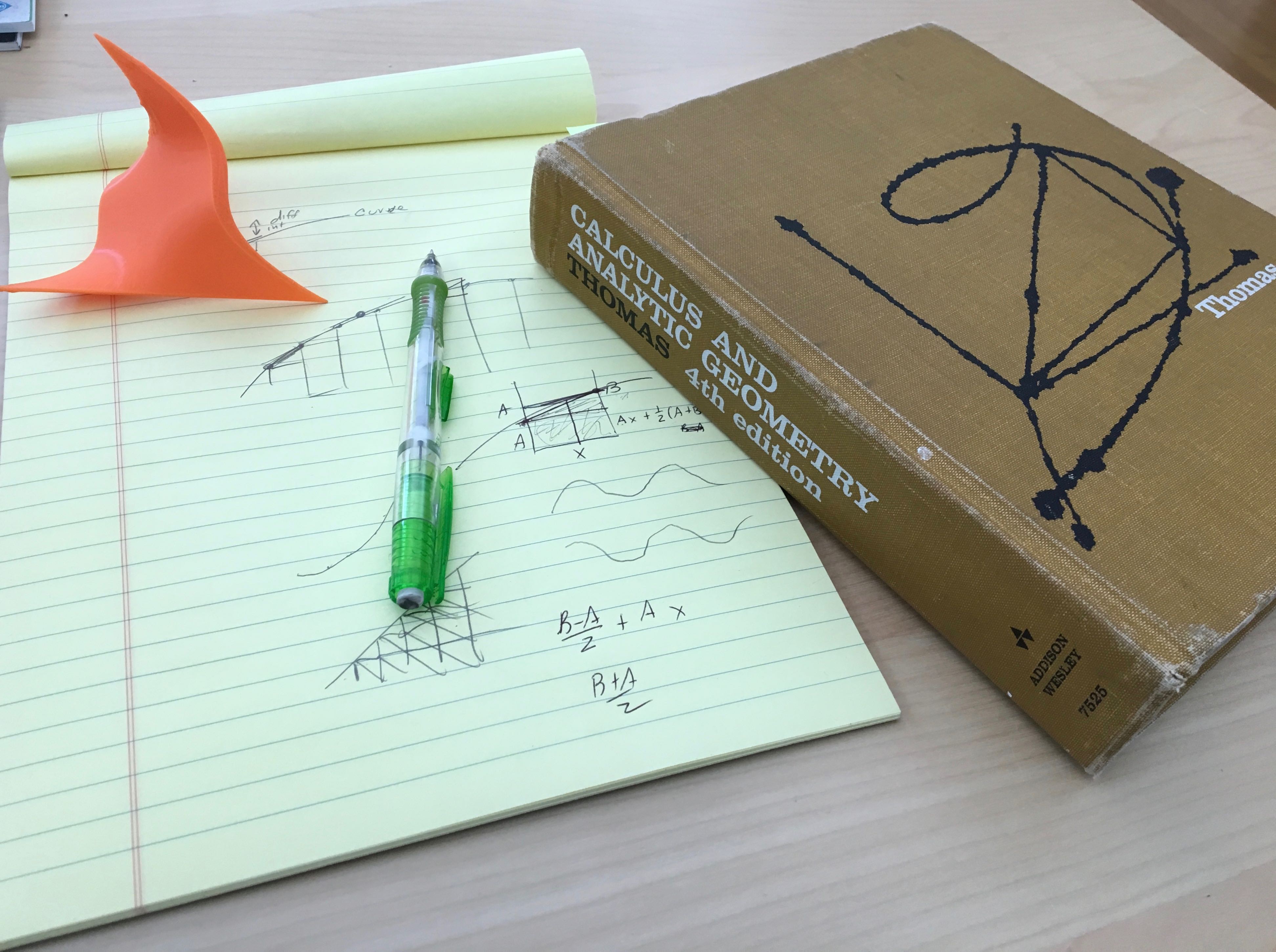
As you can see in the picture here, Joan had to party like it was 1979 with her old MIT Calculus 1 book to be sure what we're saying here is right... note the heavily-used eraser, which is always a key tool in algebraic calculus.
![Old, battred Calculus 1 text, a pad with scribbles, and a 3D print of a math function]()
Integrals
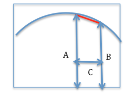
let's look at what an integral is. Most simply, in two dimensions it is a way of figuring out the area under a curve. Suppose we wanted to find the area under the curve from 1 to 2 on the horizontal axis. At point 1, the curve has the value A. At point 2, it is B. As 1 and 2 get closer together, a line drawn along the curve approximates the line more and more closely.
Suppose we wanted to find the area under the curve between the two vertical arrows marked A and B. If the red line was EXACTLY the curve, then the area would be C times the average of A and B. As the distance C gets smaller and smaller, the red line gets closer and closer to being the same as the curve. We could use a rectangle of height equal to the average of heights A and B to get the same area as finding the area under the triangle plus rectangle we'd need to figure out otherwise. You can see the diagram of this from Newton's own copy of Principia.
![]()
Suppose we also drew a line parallel to the red line. Newton found that you can always draw a line parallel to this line which is tangent to the curve. This is called the Mean Value Theorem. We will come back to that later when we talk about tying together integral and differential calculus.
The Surface
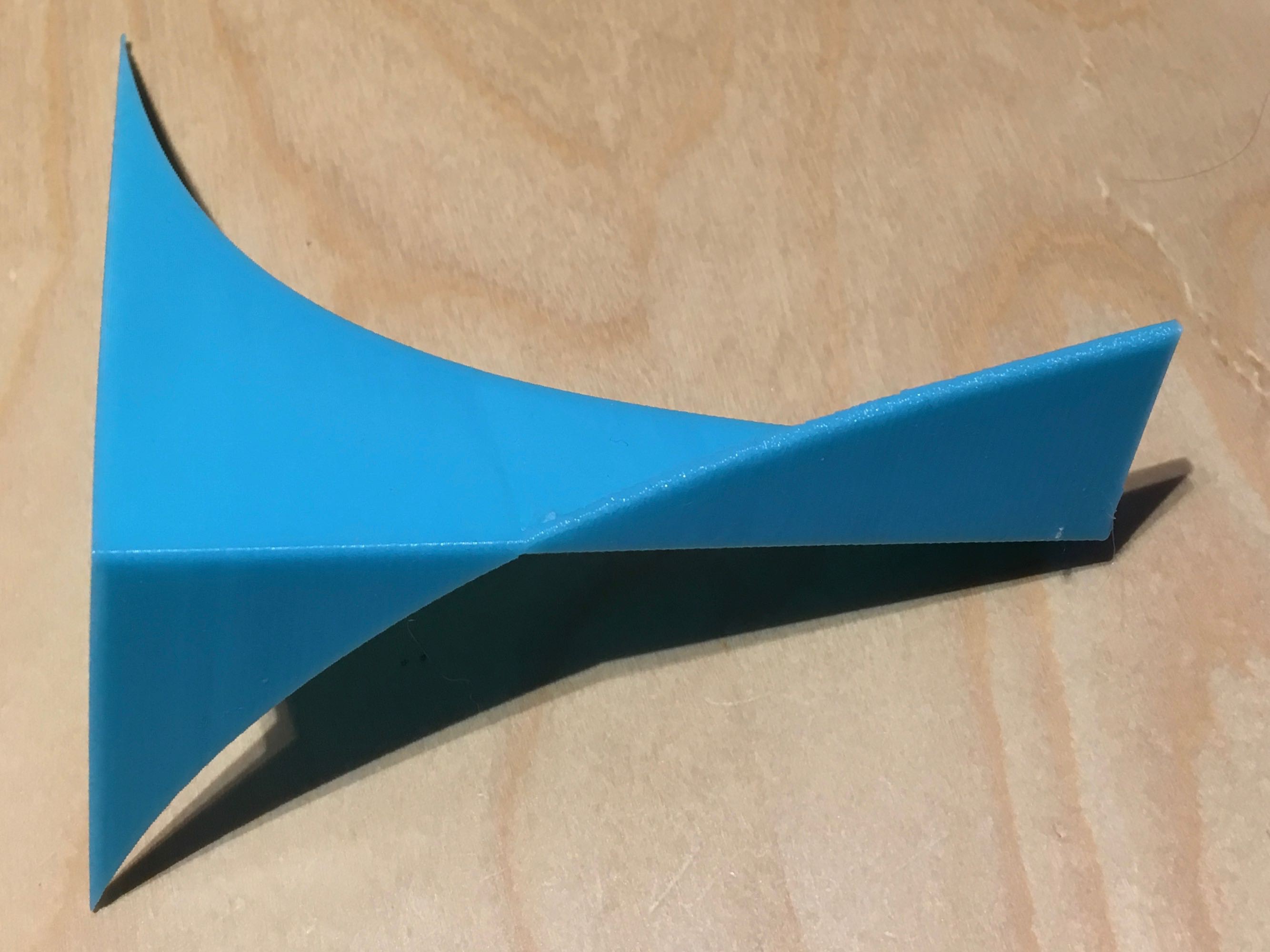
The surface we will use as an example here is called a swallowtail catastrophe. It is a surface that has some special properties that you can look into and think about a little based on what you know already, and we will use it as an example for more things to come.
The basic swallowtail equation we used was
f(x,y) = offset + ( x^5 + a * y * x^3 + b * x^2 + c * x ) / scale
Where "x^5 " means multiply x times itself five times (or, if you prefer, raising x to the 5th power), " * " means multiply, and the height of the surface is a function of two other variables, x and y. a, b, c and d are constants, and a has to be negative. For the examples we show you here, a = -10, b = c = 1.
Depending on how many data points there were, we needed to fuss around a bit with scaling and offsets so that the values of the function were always positive, since otherwise the bottom of the model would not have been a plane.
Besides having a cool name, the swallowtail is a relationship that comes up often in nature for systems that are chaotic -- acutely sensitive to initial conditions. It was also the basis for Salvadore Dali's last painting, The Swallow's Tail. (Thanks go to our mathematician friend Niles Ritter, who did his PhD thesis on related mathematics and suggested it would be a fun surface to play around with in our endeavors. Everyone else uses a paraboloid- what fun is that?)
First we will print this as smoothly as possible. It was printed with the equation printer in Chapter 1 of our 3D Printed Science Projects book; the OpenSCAD model is CC-SA-NC and available at the pubisher's repository at the same link. The surface is shown printed just in free space, and also as a surface covering a volume.
![Swallowtail function freestanding, and covering a volume over a plane.]()
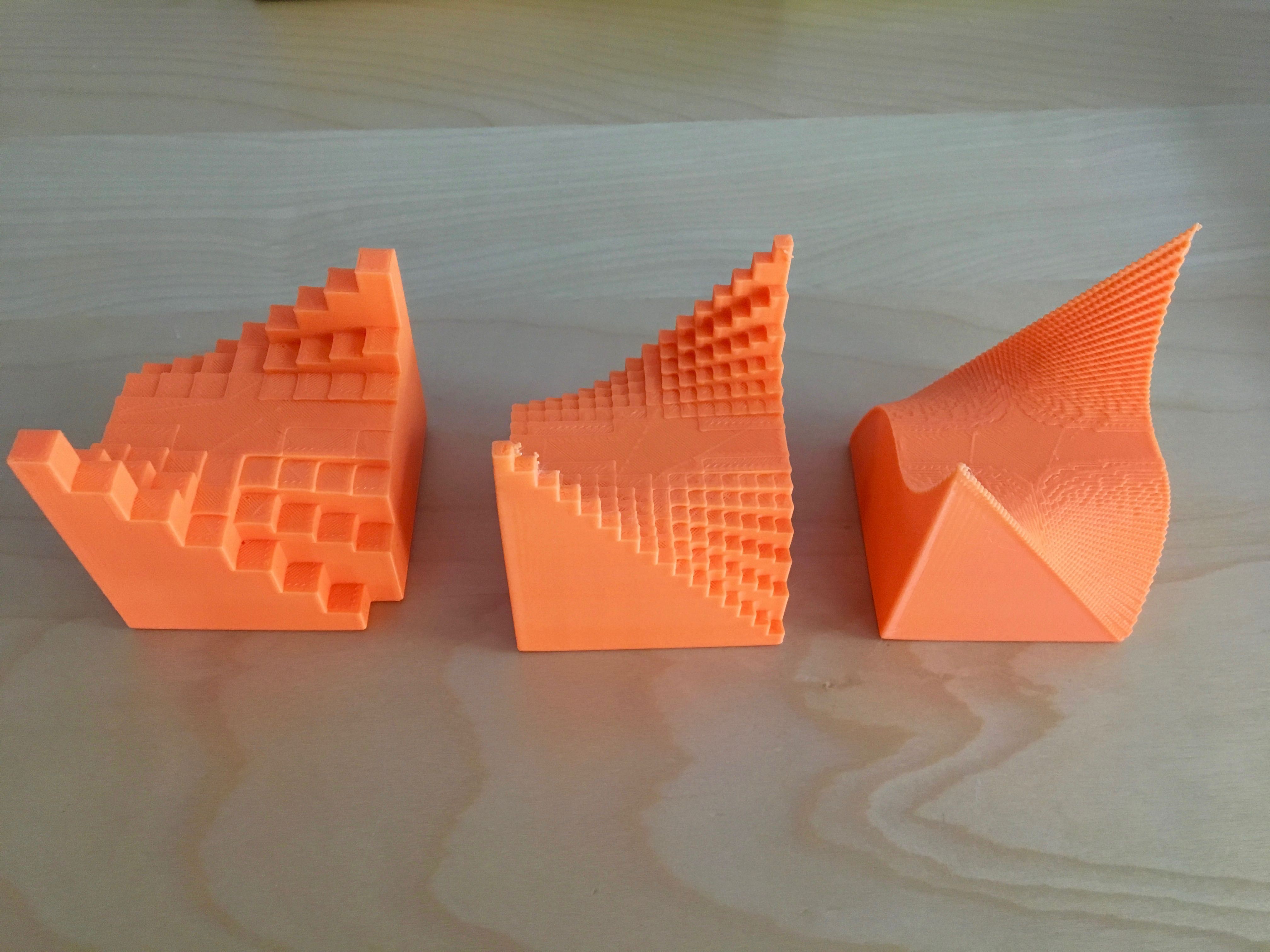
Volumes Under Surfaces
If we can get an area under a curve, it's not surprising we can do the same thing to computer the volume under a surface. Suppose we wanted to try approximating a surface by a series of rectangular solids in three dimensions and get the volume under a surface by adding up the volume of each of these rectangles. We have demonstrated this by creating little rectangular blocks with height at the mean value for a 61x61, a 16x16, and an 8x8 grid, plus the smoothest possible version. We have 3D printed all these, as you can see in the next picture. (We will post these three STLs shortly in the FILES section.)
![Three surfaces quantized progressively less coarsely, tending toward the smooth surface in an earlier picture.]()
You can see that a 61 by 61 grid is really pretty good, other than being a little rough on the surface.
How to Print a (Flock of) Swallowtails
Finally, we printed four of these at once so that those high peaks would not be distorted by overly-short times between layers. The four surfaces (the three ones with discrete rectangles, and the continuous ones) all printed in about twelve hours on a Bukito. if you printed one at a time, you'd probably have to use a cooling tower (a sacrificial tall skinny object) to keep the blobbiness at bay.
![Four swallowtail surfaces to be printed on a 3D printer.]()
So now we have seen that a derivative is just a tangent to a curve, and an integral is just an area (or volume, in 3D) under a curve. How do those relate? Stay tuned.....
-
Log #3: Research and Experiments
05/01/2017 at 00:12 • 0 commentsIn this log, we will capture some of the background research we have done so far to think about this project.
We first researched a little whether Newton had created devices himself to help him conceptualize, since he was known as a tinkerer. We have not come across any yet, but we hope to find more as we research more deeply in parallel with our experiments. There is some historic material online, but a trip to the Pasadena Public Library was required (and a bit of Amazon browsing, of course.)
The Next Device
Before we started creating the next hands-on calculus devices, we wanted to look into whether anyone had done this already. After all, for the first 200+ years of calculus' existence, there weren't any general-purpose computers. We thought we could re-create calculation aids from the 1700s or 1800s using open-source hardware and the occasional 3D printed part.
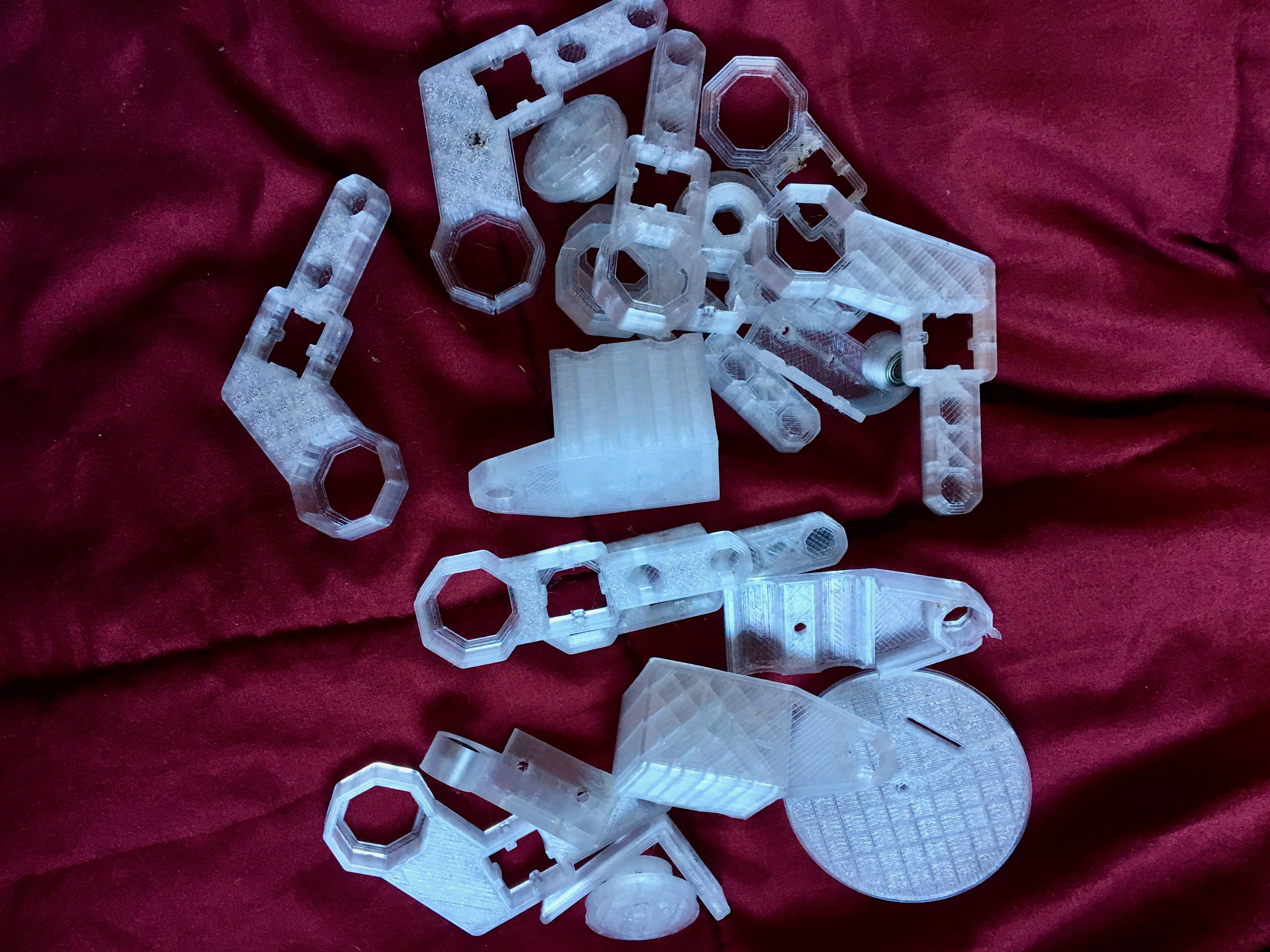
The first thing of this type we wanted to create is a device that would let the user follow a curve by hand while the device drew the derivative curve, or a mechanical differentiator. We thought there must have been mechanical devices to draw the line of the derivative of a curve, sort of the calculus equivalent of a slide rule. Surprisingly, we did not find many, or much written about using that type of device.
Here are a couple pictures of early experiments in our development of a mechanical differentiator, with 3D printed parts and pieces that will be familiar to 3D printer developers.
![Pile of iterative designs of 3D printed parts for the integrator]()
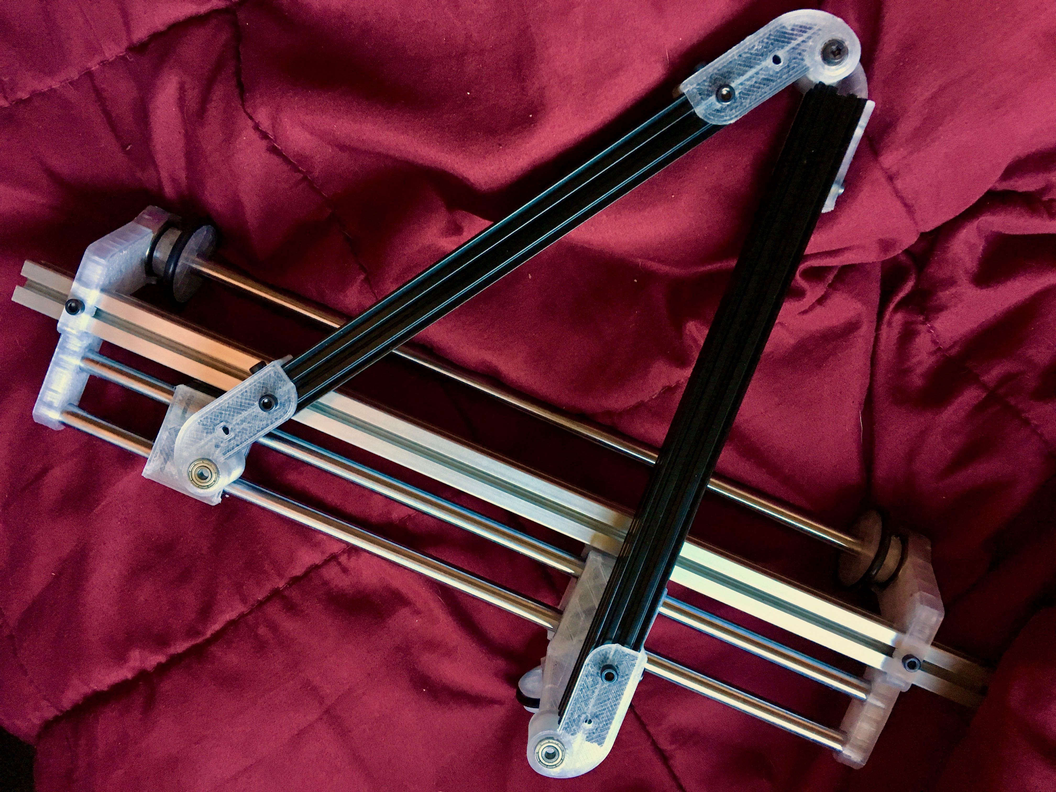
Initially we thought the device would have mostly 3D printed parts, but as it evolved it has started to look more like a chunk of a 3D printer than a 3D-printable device. As with many things, it also turned out to be harder than it looks. We will be evolving this and other devices this summer as we continue to build out this project.We'll start giving details and build instructions when our path is a little clearer - stay tuned!
![Test parts for mechanical differentiator]()
We found 1921 and 1967 patents and some descriptions in the math literature, and some interesting linkages from the late 1800s by the French mechanical designer Myard that people mentioned as a good basis for such a device, but very little about the devices.
Our conclusion is that people probably solved the problems by finding the equations for the derivative and then calculating with whatever the tools of the day were. The availability of low-cost, general-purpose computers rendered most mechanical calculating tools obsolete. But doing it that way requires you have to do the algebra before you get the intuition, which we are trying to avoid. For our purposes of building intuition, though, we think this will be the way to go, if the build doesn't get too complicated for a lot of people to make on their own.
Books, books, books
We found a version of Principia translated into modern English with commentary on what Newton would have been aware of at the time. This translation is by I.B. Cohen and A. Whitman, listing Newton as the author (University of California Press, 1999.)
Next we did some browsing to find physics or calculus taught in a similar way to what we had in mind. Not surprisingly Caltech's master physics teacher, Richard Feynman, did some lectures in the mid-1960s which were captured by the BBC and then later republished as a small book entitled The Character of Physical Law. We used the MIT Press, 24th printing in 2001, but it is available in many versions including an audiobook. It has little hand-drawn sketches and almost no algebra, and focuses mostly on gravitation. It is in many ways a modern descendant of Principia.
There is a movement generally to re-think math education in the United States. A book laying out an approach that is broadly similar to the one we suggest here is Stanford professor Jo Boaler's Mathematical Mindsets (Jossey-Bass, 2016, and summarized on the linked website.)
We are also grateful for the encouragement and ideas we're getting informally through various channels - all ideas are appreciated!
-
Log #2: Derivatives: Calculating Changes
04/30/2017 at 19:10 • 0 commentsCalculus is all about figuring out how something is changing (or how it has accumulated changes to this point). There is a lot of terminology with this that scares people off… derivatives, differential equations, integrals … but the concepts that these are shorthand for are not all that hard. We want to make this readable for people who have never seen these concepts before, and make it possible to find more online. When we define a word we think you'll want to know more about later, we'll make it a link so you can can go and read more elsewhere if this is all new to you.
The ideas apply to all kinds of changes, like pressure going up or down in a gas or stock prices rising and falling. But Newton mostly talked about actual, physical motion. Since that’s the easiest to think about for most people, that’s what we will talk about here.
Our next build (in the next few logs) will be a mechanical device that will let you graph how something is changing, which calculus would call the derivative. The process of calculating a derivative is often called differentiation. This log ties together the acceleration detector in Log #1 and our “mechanical differentiator” that we are working on in the next few logs. Later on, we are going to figure out ways to use 3D prints to visualize more complicated systems. But for now, we will go back to some very basic stuff.
Slope of a Curve
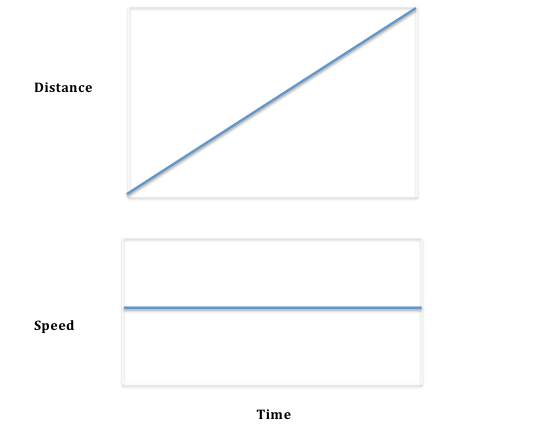
Imagine that you are running somewhere and that you always run at the same speed. You might go a tenth of a mile in a minute, have gone two-tenths in two minutes, and so on. Your distance traveled would look like this, but your speed is constant (because we said to walk that way) as we draw in the graph that follows:
![Two graphs. Top one is a straight line constantly increasing left to right, vertical axis labeled as distance and horizontal as time. Second graph is a constant line, vertical axis labeled velocity, horizontal axis as time.]()
If we asked you how fast you were running you might say “a tenth of a mile per minute” or maybe “six miles per hour.” This is the change in distance (a tenth of a mile) per change in time (a minute). Mathematicians would call this the slope of the line in the first picture – or, alternatively, the derivative of the curve in the first picture. In this case (constant speed) the slope of the whole curve is a constant and the derivative is a straight line. Let’s visualize when they are not, which was where Newton pulled together some old and new insights to create some powerful tools.
Instantaneous Slope
The example above is so easy that you are probably rolling your eyes. But suppose that the curve isn’t so simple. Look at these next two animations (done in OpenSCAD).
Notice the little line moving along the top curve. That is the instantaneous slope of the curve (it is also a line that is tangent to the curve). The bottom line is the value of that slope, just like our previous graph in this log. The little line on the bottom curve is showing that the slope is calculated from the past and current behavior of the top curve. We can't talk about change of a curve without having at least two points, although we want those points to get closer and closer together to make the slope more and more instantaneous. (There are many ways to calculate slope, but just think of this simple two-point way for now).
This first example is what it would look like if someone started out away from their house, and moved toward it and past it such that their velocity increased as shown in the lower graph. (Negative velocity we will interpret as toward the house, in this case). At the minimum point they arrive at the house, then move away again. The distance (the top line) is then a parabola.
![Paraboloa with an animated tangent line showing an instantaneous slope. A second line below shows the slope of the first curve. In this case, the slope is a straight line.]()
In this next case, someone is running back and forth, say to the right and then the left of a starting point, with their speed varying in a way we call a sinusoidal wave. The slope of a sinusoid is another sinusoid, offset in time (and sometimes scaled bigger or smaller.)
![Sinusoid with an animated tangent line showing an instantaneous slope. A second line below graps he slope of the first curve. In this case, the slope is a sinusoid, too.]()
Newton’s big insight was that if he looked at the instantaneous slope on a complicated curve (how the curve is changing if we drew a shorter and shorter slope line) he could come up with a way of describing (and then analyzing) the speed of anything, once he had a graph of how the distance varied versus time.
He was interested in how the planets moved, and he had a lot of data that had been taken by his friend and editor Edmund Halley and the earlier astronomer Tycho Brahe, plus some rules that seemed to predict planetary orbits from Copernicus and Johannes Kepler. So he had a lot of distance versus time measures (that he still had to interpret without knowing for sure how Earth was moving relatively).
Acceleration
We don't have to stop with the slope of a curve. We can take the slope of the slope- how fast our speed is changing. This is called acceleration if we are talking about motion, and in general the second derivative (the slope of the slope of a curve.) You can keep going - the third derivative is sometimes called "jerk" and is something that 3D printer designers worry about a lot.
Trying Things Out
If you take the device from log #1, you can see acceleration in the plane of the board (it ignores anything perpendicular to the board.) The red lights will "slosh" to points with more and less acceleration. Try moving your hand in a way that matches VELOCITY to the DISTANCE curve here. You can watch the brightness and direction of the red lights and think about how they are showing the derivative of the speed (not distance) of your motion.
The Mechanical Differentiator
We thought about 3D printing curves and surfaces and their derivatives, and we will set up some of that in later logs. But first, we thought a mechanical way of running a device along a curve that could draw its derivative curve would be useful. We were sure that there must have been such devices in the pre-computer era, since there are very practical applications. There sort of were; in the upcoming logs about the design process we will talk about some of them. Open-source hardware like that used for 3D printers makes assembling such a thing a lot easier than was possible in 1916, when one of the more elegant designs came along.
-
Log #1: Visualizing Acceleration
04/27/2017 at 18:31 • 0 commentsCalculus is a set of math techniques that allow us to analyze how things are changing. A lot of the explanations in Newton's original work are about how he thought about calculating relationships among a moving object's distance, speed and time.
Each of our modules will have an open-source electronics and/or 3D printing project which will help the user to learn a calculus concept, either in the build itself or by playing with the resulting object. Our first project is intended to help you get some intuition about the difference between moving at a constant speed and acceleration (speeding up, slowing down, or being affected by gravity). This first module is built around an Adafruit Circuit Playground (an Arduino-based processor with onboard sensors and programmable LEDs) to visualize interactions between gravity and a moving object.
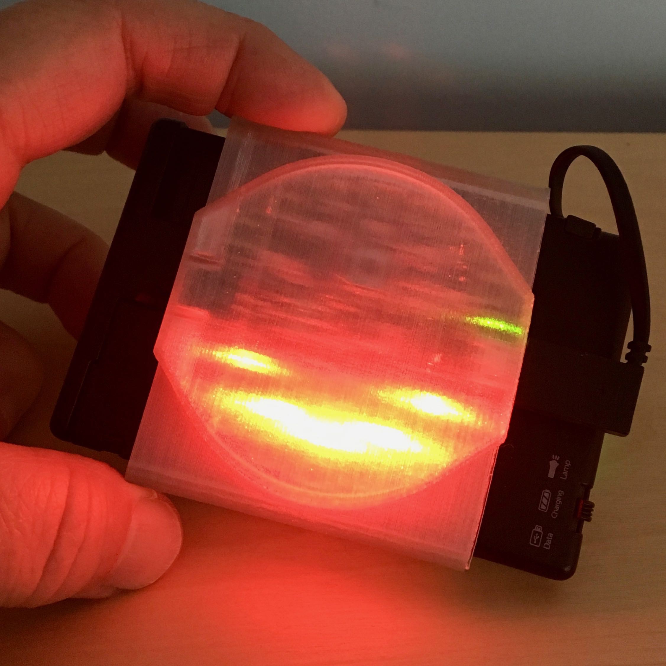
![Photo of Circuit Playground and battery in 3D printed case.]()
From here, we will build up more complicated ideas from module to module. will create different Arduino sketches to run on the hardware components described in this module.
The Concept
Calculus was invented by Newton to help him think about the motion of the planets relative to each other. One of the key things to realize if you want to understand the intuition behind calculus is that it is predominantly a way of encoding physics.
If you are standing on a planet, the force of gravity is pulling down on you. If suddenly there is no floor below you, that force opposing gravity is gone. You will start to accelerate (on earth, anyway) at 9.8 meters per second per second - so after 1 second you are going 9.8 meters per second, after two, 19.9, and so on.
These forces are what are called vectors - they have a direction. So if I am accelerating downward and also trying to speed up forward and back, I treat those separately. A device that measures that is called an accelerometer, which usually measures up and down, right and left, and front and back separately.
We wanted to design a little device that would let you play with the difference between moving at a constant speed (which does not require you to exert force) or accelerating (which does.)
The Build
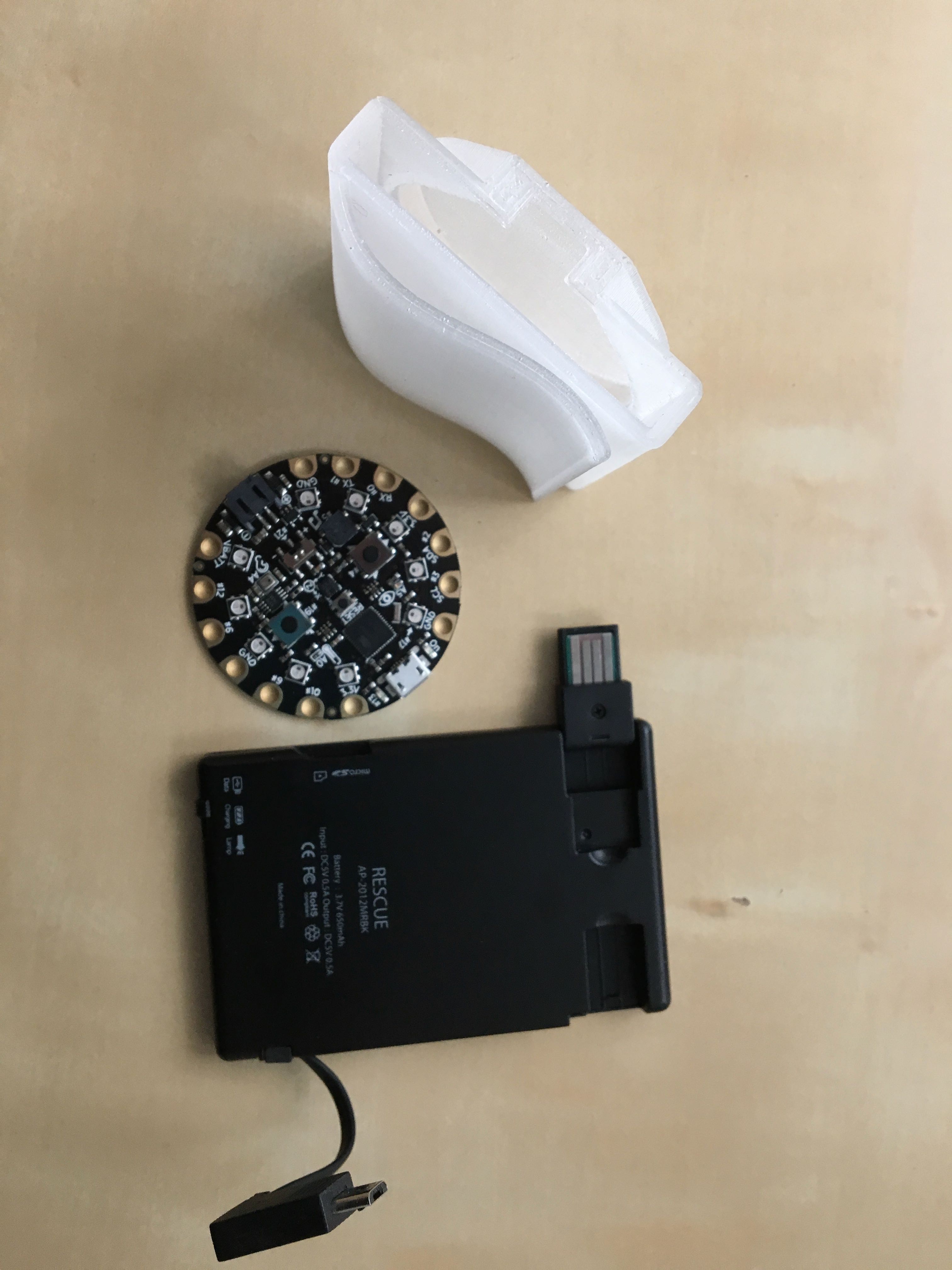
We took an Adafruit Circuit Playground, an Ares Rescue Charge Card battery, and a 3D printed case (developed by Rich, available under a CC-BY-SA license) to hold them together to create our acceleration visualizer. (Case printed in PETG for translucency). The Arduino sketch (microcontroller program) is available, also CC-BY-SA, in Rich's Github repository.
If you are new to this type of build,see the Instructions page.
The Circuit Playground has (among other things) a three-axis accelerometer, a buzzer, and programmable LEDs. Here is a picture of the 3D printed case, the Circuit Playground, and the battery.
![Components - an Adafruit circult playground board, battery, and 3D printed case]()
Assembly
The Circuit Playground fits snugly into the round part of the case, lights pointing out. The battery slides in after and locks the Playground in place.
The Arduino sketch is designed so that if the lights are pointed upward, the program will ignore gravity and only measure acceleration and deceleration in the forward-and-back and left-and-right directions. It will stay lit up green as long as you have it perfectly level. You can even (cautiously) spin it around its vertical axis and it will stay green.
Playing with Acceleration
The device will light up red and beep as soon as you turn away from level. The red lights will "fall" to the bottom of the device when it turns away from level, and small deviations from level are shown by dimming of the lights on one end. (The tolerance is a parameter in the Arduino sketch.) You can use this to anticipate that you are off-level and/or accelerating other than in the up and down direction. The device ignores vertical acceleration (that is, accelerations perpendicular to the Circuit Playground board.) This means you can accelerate and fake it out - think about how to carefully dynamically angle it to get away with that. The videos that follow show the device being moved side to side with the light appearing to slosh around.
We brought this out to World Create Day at the Pasadena SupplyFrame DesignLab and let people try to move and walk with it. Suffice it to say that there was a lot of beeping (although a few people were really good!)
We intend this version as a simple demonstration that we can build on going forward by uploading new capabilities. If you were teaching a group of people, you can use this as an icebreaker to start talking about gravity, constant velocity, and acceleration. If you are learning calculus by yourself, try out the Things To Try below. The next log will start talking about a bit more abstract stuff.
It is meant to be bright and high-contrast so that visually-impaired users will be able to see the color change unless they are completely blind. In that case, the beep will give an auditory cue, and the shape will help a user keep track of which axis is which. Suggestions on more tactile cues for the visually impaired are welcome!
Things to Try
Moving at a constant velocity and perfectly level is hard to do. Get it level (green) first and then accelerate slowly to stay under the threshold that turns it red.
Can you think of a way to accelerate slowly while walking and keeping it "level" relative to your velocity vector?
If you were an astronaut, how could you move it without beeping?
Up Next
In log #2 we will talk about distance, velocity, acceleration, and using them to understand the core concepts of calculus.
Hacker Calculus
Isaac Newton was a hacker. Let's take calculus back to its roots and make it accessible to everyone.
 Graph showing which time steps are used for each algorithm
 PID controller terms graph for stable system
 PID controller terms graph, unstable system
 PID print with a cooling tower