-
7. Conclusion
07/05/2017 at 15:29 • 0 commentsThis is a simulation-based project which aimed to model a hexapod robot in the MapleSim environment and to implement different path planning algorithms and a hierarchical control architecture. This report has presented the theoretical background, design, implementation, and control of a circular body shaped hexapod robot. The simulation model has successfully navigated between a start point and a given target point on a level terrain with randomly placed obstacles. It has been discovered and confirmed with a Maplesoft employee that the Contact Library in MapleSim is not suitable for legged-locomotion on an uneven terrain whereas wheeled-locomotion on an uneven terrain can be implemented by using the Tire Library. For that reason, an uneven terrain was constructed in the MATLAB environment and it was shown that the Footstep planner has successfully worked on an uneven terrain as well as a level terrain. Since the rest of the control hierarchy remains the same, it can be said that the provided system will potentially work on an uneven terrain.
-
6. Further Work Required
07/05/2017 at 15:22 • 0 commentsIn future, a biologically inspired self-configuration algorithm may be implemented for the cases where the robot losses one or more of its legs. Swarm Intelligence based robot reconfiguration (SIRR) method is delivered in [17]. An example is given in Figure 6.1 where hexapod reconfigures itself as a quadruped after losing Legs 1 and 5.
Figure 6.1 Robot Reconfiguration, adapted from [17]![]()
-
5. Simulation Results
07/05/2017 at 15:12 • 0 comments![]()
Figure 5.1 Omni-directional Locomotion Types, adapted from [2]
Figure 5.1 shows the 3 omnidirectional locomotion types that can be implemented in hexapod robots to change direction while navigating within an environment. MapleSim simulation environment was used for developing robot models for each omnidirectional locomotion type and for testing the hierarchical control architecture that has been presented in Chapter 4.
5.1.Centroid Rotation
Figure 5.1-a shows a hexapod robot rotating about its centre, such manoeuvrability provides a great advantage to legged robots when changing direction within a limited movement area [2]. Figure 5.2 shows the simulation results that have been generated by implementing the centroid rotation. It can be seen that hexapod robot is capable of rotating both clockwise and anticlockwise directions and it is possible to alter the step size in order to speed up the process. Notice that in Figure 5.2, the step size of the bottom hexapod is greater than the top robot.
![]()
Figure 5.2 MapleSim implementation of centroid rotation.
The 3 videos below show the MapleSim simulation results.
5.2.Slalom
Figure 5.1-b shows the slalom movement capability of the hexapod robots. The robot plans its motion as a combination of centroid rotation and straight walking. It divides its body path into linear lines and rotates about its centre between each linear line segment to align itself with the next linear region.
![]()
Figure 5.3 MapleSim implementation of slalom locomotion.
Figure 5.3 shows the slalom implementation in the MapleSim environment where the red line shows the path trace that the robot has followed. The code that was used to deduce the direction of rotation is provided in Figure 8.4 (in Appendix).
It is seen from the graph below that the robot is slightly off from the given path which is mainly a timer issue. The robot rotates about itself for 30 seconds which corresponds to about 45 degrees of rotation. This could be altered to ensure that robot follows a closer path to the blue path. However, once the dimensions of the robot is considered the robot is not that far off from the desired path.
![]()
5.3.Pedestrian-lane-change
Figure 5.1-c shows that the robot leg is moved diagonally depending on the direction of motion and the body maintains its initial orientation at all times. This particular locomotion type is named as pedestrian-lane-change by [2] and the results obtained from the MapleSim implementation are provided in Figures 5.4-5.6.
![]()
Figure 5.4 Top view of the pedestrian-lane-change locomotion.
![]()
Figure 5.5 3D view of the pedestrian-lane-change locomotion.
![]()
Figure 5.6 3D view of the pedestrian-lane-change locomotion.
![]()
Figure 5.7 The comparison of the variation in Y axis against time.
![]()
Figure 5.8 The comparison of the variation in Y axis against X axis.
Figures 5.7 and 5.8 show that the body path that the robot has followed. Considering that the wingspan of the robot is about 6 meters, the measured body path of the robot, shown in red, is almost the same as the actual body path that was calculated by body path planner, shown in blue.PRM Path Planning Implementation for Obstacle Avoidance
- Probabilistic Roadmap Method (PRM) is used to obtain a set of positions that are located on the obstacle free trajectory.
- The quintic polynomial trajectory generator uses these intermediate positions to generate the foot trajectory.
![]()
The simulation recording shows how this method works in action...
-
4. Hierarchical Control Architecture
06/30/2017 at 17:00 • 0 commentsHierarchical control architecture operates based on the sense-plan-act robot control methodology [17]. Initially, information about the surrounding environment of the robot is gathered through the sensors, then a motion plan of the next gait cycle is calculated in a goal oriented manner. Finally, the planned action is undertaken through actuators. Then the same procedure is repeated until the goal of the given task is achieved [17]. Figure 4.1 shows the block diagram of the hierarchical control architecture that is implemented in the hexapod robot. It is assumed that the terrain features are provided before the execution of the simulation.
![]()
Figure 4.1 Hierarchical Control Architecture
4.1.High Level Planner
4.1.1.Body Path Planner
For a given start point, A and a goal point, B, the shortest distance may be calculated using a map-based planning method. Note that, the shortest distance may have a higher movement cost, i.e. there might be a longer path with fewer obstacles and easier to navigate. In order to designate whether or not this is the case, the cost map of the terrain needs to be taken into account which indicates how easy the terrain is to navigate over [6]. In this report, the shortest path is assumed to be the one with the lowest movement cost.
![]() Figure 4.2-a Uneven terrain and the 2D representation of terrain, adapted from [15]
Figure 4.2-a Uneven terrain and the 2D representation of terrain, adapted from [15]Figure 4.2-a shows an uneven terrain where the regions that are higher than the reachable workspace of the robot leg, are represented as obstacles in the 2D grid that is shown on Figure 4.2-b. For example, Figure 4.3 shows a terrain height where the robot is capable of stepping over, hence in the 2D grid representation, also referred as occupancy grid, of this region is not an obstacle.
![]() Figure 4.3 Collision map of a foot trajectory over an obstacle, adapted from [28]
Figure 4.3 Collision map of a foot trajectory over an obstacle, adapted from [28] The occupancy grid framework provides information about terrain regarding to the free spaces and obstacles where each grid is roughly equal to the size of the robot. [29] For the computation, the occupancy grid is represented as a multidimensional matrix where 0 denotes free space, Qfree, and 1 denotes obstacle, Qobs [14].
The path planning algorithm, A* (star), that was implemented to compute the body path, runs in discrete space, however the real‐world is continuous hence the map needs to be discretised which is done by using an approximate cell decomposition method, trapezoidal decomposition [30]. Figure 4.4 shows the occupancy grid that was used in the MapleSim simulations. Using the trapezoidal decomposition approach, it can be decomposed into 7 cells. The idea is to extend a vertical line in Qfree until it touches either a Qobs or reaches the borders of occupancy grid [31] [32]. There is a harder-to-compute decomposition method, named as exact cell decomposition, which covers the exact shape of Qobs using convex polygons, i.e. this method produces cells with irregular boundaries. However, since all the obstacles are chosen to be rectangular, trapezoidal decomposition is sufficient enough in this particular example.
![]() Figure 4.4 Occupancy Grid Representation
Figure 4.4 Occupancy Grid Representation![]() Figure 4.5 Adjacency Map of the Occupancy Grid.
Figure 4.5 Adjacency Map of the Occupancy Grid.Then, an adjacency map is generated where each cell is represented as a node and the adjacent cells are connected with a line, shown in Figure 4.5. The adjacency map can be expressed in matrix form, where the adjacent cells are represented as 1 and the rest as 0, given by Equation 28.
![]() A* (star) path planning algorithm determines the cost of the 8 surrounding nodes by using Equation 28,
A* (star) path planning algorithm determines the cost of the 8 surrounding nodes by using Equation 28,where G is the distance from the start node and H is the estimated distance from the end node using heuristics [30]. G and H are calculated ignoring the obstacles, where the vertical and horizontal movements are counted as increments of 1 whereas the diagonal motions are counted in increments of √2. Table 3-1 shows an example of how G and H were calculated for Nodes A, B, and C that are shown on Figure 4.6. The nodes with the lowest cost, F, are given priority in the exploration process.
![]() Table 3‑1 Example G, H, and F values of Nodes A, B, and C.
Table 3‑1 Example G, H, and F values of Nodes A, B, and C.![]() Figure 4.6 The body path found by the A* algorithm MATLAB Script 8-3 (in Appendix) was used to generate the path in Figure 4.6 which shows the generated body path between Start node and Goal node in grey and the obstacles are shown in black. It can be seen that, the path given in Figure 4.6 is not smooth. In order to obtain a smoother body path, a 2nd order low pass Butterworth filter is applied and hence, the body path given in Figure 4.7 is generated. This path has been used in the MapleSim simulations as the test body path.
Figure 4.6 The body path found by the A* algorithm MATLAB Script 8-3 (in Appendix) was used to generate the path in Figure 4.6 which shows the generated body path between Start node and Goal node in grey and the obstacles are shown in black. It can be seen that, the path given in Figure 4.6 is not smooth. In order to obtain a smoother body path, a 2nd order low pass Butterworth filter is applied and hence, the body path given in Figure 4.7 is generated. This path has been used in the MapleSim simulations as the test body path.![]() Figure 4.7 The body path that is used in the MapleSim simulations
Figure 4.7 The body path that is used in the MapleSim simulations4.1.2.Footstep Planner
The footstep planner, provides the initial configuration, , and final configuration, that are required by the foot trajectory planner to generate the trajectory that traverses from to where is the current foot position and is the position of the next footstep [16]. The footstep planner makes a projection of where the leg end effector needs to be positioned for the next step in order to follow the path that was given by the body path planner [18].
![]() Figure 4.8 X-Y View of the possible Final Foothold Configurations.
Figure 4.8 X-Y View of the possible Final Foothold Configurations. Figure 4.8 illustrates the reachable area of the leg end effector in the increments of 10 degrees where the Z axis was kept constant at -1 in order to represent a level terrain. Since it is assumed that the robot only moves forward and sideways but not backwards, the possible final foothold configurations that can be chosen by the footstep planner are limited by the area that is given by Figure 4.9.
![]() Figure 4.9 X-Y View of the possible Final Foothold Configurations in the 1st Quadrant.
Figure 4.9 X-Y View of the possible Final Foothold Configurations in the 1st Quadrant. The procedure to compute the final configuration, qf is as follows. The derivative of the path signal that is given by the body path planner is computed with respect to time to obtain the slope, α(t) as a function of time. Then, the signal is amplified by a gain, G which was selected such that the maximum value of α(t)corresponds to π/2 where the robot moves vertically. Equations 29 and 30 are used to calculate the Cartesian coordinates, and of the next final foothold configuration such that the robot follows the given body path.
where R is a constant that specifies how much further the end effector will be positioned from the fixed frame of the individual leg. In the MapleSim simulations, R is chosen to be 1.2 due to the torque constraints on the joint actuators, hence the actual operational area of the leg end effector is the area that was enclosed by the black dashed line shown in Figure 4.9. Figure 4.10 shows 4 different leg configurations and the corresponding horizontal distances to the geometric centre of the body.
![]() Figure 4.10 Different leg configurations and corresponding R values of the MapleSim Model.
Figure 4.10 Different leg configurations and corresponding R values of the MapleSim Model.The Z coordinate of the qf is a matter of altitude which is obtained by finding the corresponding height of the point from the height map of the terrain for any given X and Y coordinates. Figure 4.12 shows the possible positions on an arbitrarily generated uneven terrain such that the chosen random variables lie within ±0.25m of the exponential function given by Figure 4.11 which represents a hill.
![]() Figure 4.11 Curve that was used to generate the uneven terrain
Figure 4.11 Curve that was used to generate the uneven terrainFigure 4.12 3D View of the possible final foothold configurations on an uneven terrain
![]()
Figure 4.12 3D View of the possible final foothold configurations on an uneven terrain
Figure 3.13 shows the X-Y view of the positions of qf on an arbitrarily generated height map, it can be seen that the X axis was incremented by 0.1m in order to reduce the computation time. MATLAB Script 8-4 (in Appendix) was used to create the uneven terrain that is shown in Figure 4.12.
![]() Figure 4.13 X-Y view of the final foothold configurations on an uneven terrain
Figure 4.13 X-Y view of the final foothold configurations on an uneven terrain4.2.Low Level Planner
4.2.1.Foot Trajectory Planner
![]()
The kinematic analysis of a robot manipulator is concerned with the geometry of the robot and the constraints due to the existence of an obstacle within the workspace of the robot leg are completely neglected. The possibility of collisions is taken into account by the foot trajectory planner and a collision free path is generated [16].
The foot trajectory planner computes the dynamics of the leg end effector motion during the swing phase as it traverses from an initial configuration, qo, to a given final configuration, qf [16]. Table 3-2 gives the notations that are used in this section of the report.
Figure 4.14 shows a foot trajectory which is decomposed into 3 sections labelled as 1, 2, and 3, respectively. During section 2, the leg moves faster whereas in sections 1 and 3, the leg moves slower to avoid an impact with the ground. Therefore, a minimum number of 4 constraints; initial configuration, qo, final configuration, qf, initial velocity, vo, and final velocity vf needs be taken into account.
![]() Figure 4.14 Foot Trajectory between initial and final configurations.
Figure 4.14 Foot Trajectory between initial and final configurations.![]()
MATLAB Script 8-5 (in Appendix), was used to calculate the position, velocity and acceleration of each joint of Leg 1. Figure 4.15 demonstrates the variation in position, velocity and acceleration of Joints 1, 2, and 3 during a complete leg cycle of 4 seconds.
The velocity plots, in Figure 4.15, show that velocity of joints peaks at the centre of each one-second segment. In other words, for the majority of the time, the velocity is below its maximum value which is inefficient and hence undesirable. In order to solve this problem, linear segment with parabolic blend (LSPB) method was implemented which has increased the duration for which the joint operates at its maximum velocity [14]. Figure 4.16 shows the position, velocity and acceleration profiles calculated by LSPB method and the code is given in MATLAB Script 8-6 (in Appendix).
![]()
Figure 4.15 Position, Velocity, and Acceleration profiles for Quintic Polynomial
![]()
Figure 4.16 Position, Velocity, and Acceleration calculated by the LSPB Planner
It can be seen in Figure 4.17 that the trajectory of the complete leg cycle is linear since all the intermediate velocities between consecutive segments were set to 0ms-1. Using heuristics, the optimum intermediate velocities may be calculated given that only initial and final velocities are 0ms-1. Figure 4.18 shows the position, velocity, and acceleration calculated using heuristics, notice that the intermediate velocities are no longer equal to 0ms-1. Consequently, the generated foot trajectory, shown by Figure 4.19, is an arc instead of a straight line as it was shown in Figure 4.17. MATLAB Script 8-7 (in Appendix) was used to generate Figures 4.17 and 4.19.
![]() Figure 4.17 The Foot Trajectory generated using the LSPB Planner
Figure 4.17 The Foot Trajectory generated using the LSPB Planner![]() Figure 4.18 Position, velocity, and acceleration calculated using heuristics
Figure 4.18 Position, velocity, and acceleration calculated using heuristics![]() Figure 4.19 The Foot Trajectory generated using heuristics
Figure 4.19 The Foot Trajectory generated using heuristics![]() Figure 4.20 MapleSim implementation of the generated trajectory
Figure 4.20 MapleSim implementation of the generated trajectoryFigure 4.20 shows the simulation of the foot trajectory which was obtained using quantic polynomial that is given by Equation 31. Notice that, during the swing phase, the leg end effector approaches the body in the direction of axis, shifting the mass towards the COG, reduces the mass distribution and hence minimises the angular momentum [33]. Due to the law of conservation of total momentum, the reduced angular momentum must be compensated by the speed of the motion i.e. the end effector pursues on the given trajectory at a higher velocity [33].
When the robot is navigating on an uneven terrain, a path planner algorithm needs to be implemented in order to compute the Cartesian coordinates of the end effector for a given number of intermediate segments within the trajectory. These Cartesian coordinates are then connected and a collision-free trajectory is obtained.
As it was mentioned in the literature review, artificial potential fields, probabilistic roadmap method (PRM) and rapidly exploring random trees (RRT) algorithms are widely used to generate a point-to-point trajectory [12] [16] [7]. Using artificial potential fields may be quite problematic since the existence of a local minima in the field causes the algorithm to get trapped [16]. As a result, random motion algorithms appear to be better alternatives since these algorithms are often quicker in terms of computation [16]. The PRM algorithm is more advantageous over RRT which spreads omni-directionally, mainly because relatively fewer points need to be tested in order to generate the trajectory between initial configuration, qo, and final configuration, qf, which reduces the computation time. Computation time needs to be taken into account since this process is repeated in every footstep and hence an algorithm that creates less computational burden was chosen [14].
![]() Figure 4.21 Arbitrarily generated obstacle to test the PRM algorithm
Figure 4.21 Arbitrarily generated obstacle to test the PRM algorithmFigure 4.21 shows an obstacle that is located within the configuration space of the robot,. An occupancy grid matrix is generated in a similar manner to the body path planner where the is discretised by representing the obstacle region, Qobs, as 1 and free configuration space, Qfree, as 0.
Equation 38 illustrates the occupancy grid of the obstacle shown in Figure 4.21 using a 10 by 10 matrix, the matrix dimension may be extended to 100 by 100 to improve the accuracy however the computational burden on the processor would be increased as a trade-off. Notice that the matrix given by Equation 38 is vertically inverted since the 1st row and 1st column corresponds to the origin (0,0) of the Cartesian coordinate system.
![]() The chosen path planner algorithm, PRM, generates a set of random configurations within Q then the end effector configurations that lie within Qobs are neglected and the configurations that are located within the borders of the Qfree are connected by straight lines to form pairs of configurations given that the lines do not violate the Qobs [16]. The lines that introduce a collision, i.e. violate the Qobs are also neglected. Then, the Cartesian coordinates of the configurations that are located on the shortest roadmap connecting the qo and qf are used by the trajectory planner to generate the collision free foot trajectory that lands on the position projected by the footstep planner. Figure 4.22 shows the set of configurations that needs to be followed to prevent a collision with the arbitrarily generated obstacle, where the randomly chosen configurations are denoted by blue nodes and the configurations that lie on the shortest roadmap are denoted by green nodes. In this particular example, the qo and qf are chosen as (2,1) and (9,1), respectively, whereas in the simulation the initial and final configurations are provided by the footstep planner.
The chosen path planner algorithm, PRM, generates a set of random configurations within Q then the end effector configurations that lie within Qobs are neglected and the configurations that are located within the borders of the Qfree are connected by straight lines to form pairs of configurations given that the lines do not violate the Qobs [16]. The lines that introduce a collision, i.e. violate the Qobs are also neglected. Then, the Cartesian coordinates of the configurations that are located on the shortest roadmap connecting the qo and qf are used by the trajectory planner to generate the collision free foot trajectory that lands on the position projected by the footstep planner. Figure 4.22 shows the set of configurations that needs to be followed to prevent a collision with the arbitrarily generated obstacle, where the randomly chosen configurations are denoted by blue nodes and the configurations that lie on the shortest roadmap are denoted by green nodes. In this particular example, the qo and qf are chosen as (2,1) and (9,1), respectively, whereas in the simulation the initial and final configurations are provided by the footstep planner.![]() Figure 4.22 The intermediate end effector positions that connect qo and qf.
Figure 4.22 The intermediate end effector positions that connect qo and qf.The PRM planner needs to be specified with a safety margin, i.e. minimum distance that the green nodes can be positioned. An example is shown in Figure 4.23. In practice, a zone surrounding the obstacle is formed which the planner treats as an expanded Qobs and hence it will not be violated. To illustrate, the node that is located on (4,5) is not chosen by the planner since its location lies within the specified safety margin of 0.3m.
![]()
Figure 4.23 [6] Safety margin.
![]()
Figure 4.24 The complete foot trajectory
Figure 4.24 shows the generated foot trajectory by using the intermediate leg configurations that were given by the PRM Planner. This trajectory is used to compute the 3 joint angles, θ1, θ2, and θ3 by using the inverse kinematics equations to make the leg step over the obstacle and land to the projected .
Figure 4.45 shows the simulation result that was generated in the MapleSim environment. The black line shows the path trace of the motion and it can be seen that the leg steps over the obstacle as expected. The same method is used by the hexapod robot to compute the trajectory over an obstacle while navigating on an uneven terrain.
![]()
Figure 4.25 MapleSim implementation of the generated foot trajectory
4.2.2.Body Trajectory Planner
As it was stated in Section 3.2., the adapted walking gait and dynamic stability approaches are used by the MapleSim model to maintain the stability of robot when the terrain becomes steeper or the locomotion speed is increased so that the static stability may no longer be preserved. The results showed that the dynamic stability approach appears to be more advantageous over adaptive walking gait since it improves the locomotion speed of the robot while maintaining its stability.
Adaptive Walking Gait Selector
In the MapleSim simulation, the SM of the motion, which is an indication of how close the robot is to be statically unstable, was used to alter the walking gait depending on the slope of the terrain that the robot is located on. For instance, the walking gait is switched from tripod gait to wave gait in order to increase the area of the support polygon and hence the stability of the robot.
Figure 4.26 shows the support polygon that is formed between the ground contact points during wave gait where a single leg is in the swing phase at a time. It can be seen that the wave gait is intrinsically more stable since the area of the support polygon is greater comparing to tripod gait. Figure 4.27 shows the transition from tripod gait to wave gait to improve the stability. However, note that, this transition gave rise to a trade-off between locomotion speed and stability as it is shown in Figure 3.23-c. The MapleSim code that was used to generate the adaptive walking gait is shown in Figure 8.2 (in Appendix).
![]()
Figure 4.26: Bottom view of the Hexapod Robot during wave gait
![]()
Figure 4.27 The transition from tripod gait to wave gait.
![]()
Figure 4.28 The variation in SM when the walking gait is changed.
Figure 4.28 shows that the SM has increased when the walking gait is changed to wave gait, indicating that the robot is less expected to lose its stability.
Dynamic Stability
The static stability criterion that was covered in Section 3.2 does not take the effect of external forces into account which are caused by the inertial acceleration of the robot. For a legged robot that is navigating on an uneven terrain, the vertical projection of the COG is expected to be located outside or on the border of the support polygon [20].
Therefore, dynamic stability criterion needs to be implemented which is based on computing the optimum acceleration profile of the COG that keeps the zero moment point (ZMP) within the borders of the support polygon during a complete gait cycle [34] [18]. In other words, even though the vertical projection of the COG is located outside the support polygon, the robot is balanced by the external forces that are created during motion. ZMP is defined by [35] as "the point on the ground surface about which the horizontal component of the moment of ground reaction force is zero.” The position of the ZMP, coincides with the position of the COG when the robot is stationary where COG is assumed to be located at the geometric centre of the robot [34] [30].
The body trajectory planner, say in tripod gait, takes the estimated positions of the next 3 footholds which were calculated by the foot step planner and computes a COG trajectory given that ZMP of the robot is kept within the support polygon [18]. The relationships between the position of the ZMP along the X axis, x_ZMP and the Y axis, y_ZMP are given by Equations 39 and 40, respectively.
where xm, ym and zm are the X, Y and Z coordinates of the COG and g is the gravitational acceleration [18].
![]() Figure 4.29 The trajectory of COG and ZMP during tripod gait, adapted from [18]
Figure 4.29 The trajectory of COG and ZMP during tripod gait, adapted from [18]Figure 4.29 shows the trajectory that the COG traverses from previous support polygon to next support polygon while ZMP is kept within the current support polygon which is shown by the black triangle [18].
4.3.Low Level Controller
In real life, the planned footstep placement and foot trajectories may not be executed as anticipated due to a number of affects such as friction, jamming, slippage, and meshing. Consequently, the stability of the robot is jeopardized and hence the robot locomotion is no longer accurate. In order to overcome the mentioned problems, 2 low level controllers are implemented [18].
4.3.1.Inverse Dynamics
Inverse dynamics is a nonlinear control technique that provides a better trajectory tracking by calculating the required joint actuator torques that need to be generated by the motors to achieve a given trajectory [25] [16].
As it is given in Section 3.4.1, the matrix form of the dynamics of a robot leg is given by Equation 41 where the F and J terms are neglected [25].
For a given q0 and v0 the nonlinearity of the system can be vanished, making the system linear and hence the exact amount of torque that needs to be generated by the joint actuator to overcome the inertia of the actuator can be calculated. If the q0 and v0 match with the desired q0 and v0 then the projected trajectory will be tracked as expected [35].
Equation 42 shows the control law expression where is a^q new input to the system. The numeric value of a^q is calculated by Equation 43 where q_d is the desired trajectory, q is the actual trajectory, and Kp and Kd are position and velocity gains, respectively [16].
Since the mass matrix, M, is invertible, equating Equation 41 to Equation 42 gives the expression in Equation 44 which shows that the new system is linear as it is given by Equation 45.
Figure 4.30 demonstrates the inner loop and outer loop control architecture where the output of the system yields the joint space signal which enables a better trajectory tracking given that the feedback gains Kp and Kd are tuned as appropriate.
![]() Figure 4.30: Inner Loop – Outer Loop Linearized Control, adapted from [16]
Figure 4.30: Inner Loop – Outer Loop Linearized Control, adapted from [16]4.3.2.Stability Detection and Recovery
![]()
Figure 4.31: The foot positions that are likely to cause a slippage, adapted from [2]
Figure 4.31 shows the foothold positions that the robot leg may slip during the stance phase. Figure 4.31-b has a higher chance of slippage than the foot positions that are shown in Figure 4.31-a. For such cases, a recovery controller needs to be implemented for real life applications where conditions are not ideal, this controller is particularly suitable for the cases in which the robot slips or an unexpected obstacle happens to be present within the workspace of the robot leg. The recovery controller provides a reflex based reaction to the 3 cases that are shown in Figure 4.32.
- In Figure 4.32-a, the leg slips from position 1 to position 2 then the recovery controller takes action and leg is moved to position 3 to minimise the slippage.
- In Figure 4.32-b, the leg encounters an unexpected obstacle at position 2 and leg is raised higher to overcome the obstacle and positioned to position 3.
- In Figure 3.32-c, no contact is detected at the expected location 2 and the leg seeks for another foothold and eventually detects position 3.
![]()
Figure 4.32: Recovery reflexes, adapted from [4]
-
3. Fundamentals of Hexapod Robot
06/29/2017 at 15:01 • 4 commentsIn this chapter, the fundamental concepts of hexapod robots such as walking gaits, stability, kinematics and dynamics are covered which are essential to obtain a better understanding of the control architecture that is delivered in the next chapter.
3.1.Walking Gaits
In this section, the phases in a leg cycle are introduced, then different gaits are covered and simulations results are represented.
3.1.1.Swing and Stance phases of a Hexapod
Figure 3.1 shows the swing and stance phases of a robot leg cycle. A leg cycle is the combination of raising and placing a leg and it consists of 2 stages: the swing phase and the stance phase. During the swing phase, the leg traverses from the initial position to final position through air, shown by blue dashed line. On the other hand, during the stance phase, the leg end effector is in ground contact while the leg traverses from the final position to the initial position, moving the robot in the opposite direction to the red arrow.
![]()
Figure 3.1 Robot leg cycle divided into swing and stance phases, adapted from [20]
3.1.2.Tripod Gait, Wave Gait, and Ripple Gait
There are 3 walking gaits that are commonly observed in the nature: wave gait, ripple gait, and tripod gait. The tripod gait was covered in the progress report which is provided in the Appendix 8.3. Wave gait is the slowest in terms of the locomotion speed, yet the most stable. In the wave gait, only 1 leg is in the swing phase at a time while the other 5 legs are in the stance phase. The locomotion speed of ripple gait is slower than tripod gait nevertheless it is faster than the wave gait, since 2 legs from opposite sides are in the swing phase by 180 degrees offset, at a time. These 2 walking gaits are shown in Figure 3.3 where the solid lines and dashed lines represent the swing phase and stance phase, respectively [17]. Figure 3.2 shows the numbering of the hexapod robot legs where the red arrow specifies the front of the robot that was created in the MapleSim environment.
![]()
Figure 3.2: Top view of the robot model that was used in the simulations
![]()
Figure 3.3 Sequence of swing and stance phases in walking gaits, taken from [17]
3.2. Stability in Hexapod Robots
The stability of legged robots is divided into two categories: static stability and dynamic stability. To be considered statically stable, the robot needs to be stable during its entire gait cycle, without the requirement of any force to balance the robot [20]. While the robot is statically stable, the vertical projection of its centre of mass (COM) is located within the support polygon which is formed between the legs that are in the stance phase. In the case of COM being positioned on the border or outside the support polygon, the robot falls over unless it is dynamically stable, i.e. robot is balanced while walking due to the inertia caused by the motion and is statically unstable when it stops moving [21]. Figure 3.4 demonstrates the support polygon of the MapleSim model during tripod gait where the red circle denotes the vertical projection of its COM.
![]()
Figure 3.4 The Support Polygon that is formed During Tripod Gait.
Figure 3.5 shows the bottom view of the hexapod robot where the support polygon is decomposed into 3 sub-triangles in order to calculate the Stability Margin.
![]()
Figure 3.5 The Bottom View of the Support Polygon Decomposed into Sub-triangles.
Following [22], the area of the convex pattern between Leg 1, Leg 5 and the projection of COM is calculated by Equation 1.
S1= 1/2 |(X1-Xc)*(Y5-Yc)-(X5-Xc)*(Y1-Yc)| (1)The distance between two ground contact points of Legs 1 and 5, is calculated by Equation 2.|L1|=√((X5-X1)^2+(Y5-Y1)^2 ) (2) h1=(2*S1)/|L1| (3)Since the area of a triangle is the product of base and height divided by two, the perpendicular distance,, from the vertical projection of COM to L1 is given by Equation 3. Figure 3.6 shows the heights of the 3 sub-triangles.![]()
Figure 3.6 Heigths of the sub-triangles
Then, the same process is repeated to calculate S2, h2, S3 and h3. Stability margin (SM) is the shortest distance between the position of COM projection and the support polygon borders [20]. In this particular example, SM is equal to . The mathematical expression for SM is given by Equation 4.
SM=min(h1,h2,h3) (4)The state of variable indicates whether or not the robot is statically stable. The mathematical expression for is given by Equation 5,T=1 if Sk=A (5) T=0 if Sk≠A (6)where n is the number of legs in stance position at a given time and A is the area of the entire support polygon. Figure 3.7 shows the variations in SM while the robot follows the body path that is used in the experiments shown in red. The MapleSim code that was used to calculate the SM, is shown in Figure 8.2 (in Appendix).![]()
Figure 3.7 Variation in the SM while the robot is following the given body path
The variable was used in the simulation to terminate the process if the robot becomes statically unstable. Although, this is not a concern in the level terrain, when the robot navigates on an incline surface as it is demonstrated in Figure 3.8, the vertical projection of the COM is closer to the borders of the support polygon, making the robot more likely to be statically unstable. There are two ways to solve this problem. The first one is to implement an adaptive gait generation and the second one is to make the robot dynamically stable. These two proposed solutions are tested in the MapleSim environment and the findings are presented in Section 4.2.2.
![]()
Figure 3.8: Side view of the hexapod model on an incline surface of
![]()
Figure 3.9: Front view of the hexapod model on an incline surface of
Figure 3.9 shows how θ3 of Joint 3 is altered to ensure that Link 3 is perpendicular to the horizon, this is achieved by an geometric approach where the roll angle of the body was measured by an Euler Sensor. Then, the output from the sensor, γ was added to or subtracted from θ3 that was calculated by the inverse kinematic equations, depending on the direction of the robot. The block diagram of the procedure is shown in Figure 3.10. An analytical approach can be found in [23].
![]()
Figure 3.10: Posture Control – Block Diagram.
3.3.Kinematics of Hexapod Robot
3.3.1.Forward Kinematics
The forward kinematics is used to derive a set of kinematic equations that yields the position and the orientation of the robot end effector for the given joint parameters of the robot manipulator [16]. The derived equations were used by the footstep planner to compute the workspace of the robot leg and to project potential final configurations for the robot end effector. Denavit-Hartenberg (DH) convention states that each homogeneous transformation, Hi, can be expressed as a product of 4 transformations, given by Equation 6,
Hi=R(Zi,θi) T(Zi,di) T(Xi,ai) R(Xi,αi) (6)where R and T denote rotation and translation, respectively [16]. Equation 7 shows the matrix that has been calculated from the product of 4 transformation matrices given in Equation 6.
Equation 7 can be expressed in the matrix form which is given by Equation 8.![]()
The homogeneous transformation between the fixed frame and the end effector for a 3 DOF robot manipulator![]()
is calculated by multiplying the transformation matrices between each joint,
given by Equation 9 [24].
Figure 3.11 demonstrates the leg of simulation model that was developed in the MapleSim environment and Figure 3.12 shows the corresponding diagram that was used to obtain the DH Parameters.
![]()
Figure 3.11: Simulation Model Leg
The DH Parameters of each leg is given by Table 2-1
![]() Table 2‑1 DH parameters
Table 2‑1 DH parameters ![]() Figure 3.12 Forward kinematic model of the robot leg
Figure 3.12 Forward kinematic model of the robot leg In order to verify the obtained DH Parameters, MATLAB Script 8-1 (in Appendix) was used to calculate the end effector coordinates of the robot leg when it is in the rest position, i.e. θ1, θ2, and θ3 are equal to 0 degrees. Equation 10 shows the calculated Cartesian coordinates, using MATLAB Script 8-1, which are the same as the coordinates of the end effector, shown in Figure 3.13 confirming the DH Parameters to be correct.
![]() Figure 3.13 Hexapod leg in rest position
Figure 3.13 Hexapod leg in rest positionThe DH Parameters that are shown in Table 2-1 are used to visualise the reachable workspace of the robot leg. Figure 3.14 illustrates the 3D view of the end effector positions and Figure 3.15 illustrates the side views where; θ1 was altered from -90 to 90 in increments of 10 degrees, θ2 was altered from -90 to 90 in increments of 15 degrees, and θ3 was altered from -60 to 135 in increments of 15 degrees. MATLAB Script 8-2 that is provided in the Appendix, was used to generate Figures 3.14 and 3.15.
![]() Figure 3.14 3D view of the reachable workspace of robot leg
Figure 3.14 3D view of the reachable workspace of robot leg![]() Figure 3.15 X-Y and Z-X views of the reachable workspace of robot leg
Figure 3.15 X-Y and Z-X views of the reachable workspace of robot legThe same approach can be applied to calculate the combinations of revolute joint angles, θ1, θ2 and θ3 that cause a collision with an obstacle that is located within the workspace of the robot leg. Figure 3.17 demonstrates the angles combinations that the leg end effector collides with the obstacle shown in Figure 3.16.
![]() Figure 3.16 MapleSim Model and Obstacle located within the Workspace of Leg 3.
Figure 3.16 MapleSim Model and Obstacle located within the Workspace of Leg 3.![]() Figure 3.17 The combination of angles that cause a collision with the Obstacle.
Figure 3.17 The combination of angles that cause a collision with the Obstacle.3.3.2.Inverse Kinematics
As the complexity of the system increases, the robot is desired to undertake as many calculations as possible since the computation capabilities of human operator is limited. [12] Similarly, calculating the angle of joint rotation for 6 legs in order to move the hexapod robot from position A to position B is a challenging task for the operator therefore, the robot is required to compute this calculation and be capable of moving the end effector of the robot legs to the given coordinates. This task is handled by inverse kinematics equations in which the joint angles are calculated that will make the end effector achieve the particular X, Y, and Z coordinates. [39] The derivation of equations are as follows:
![]()
Figure 3.3.1 Top view of a single robot leg
Figure 3.3.1 shows the top view of a single robot leg. An axis is defined in the direction of the leg and it is labelled as ρ. The coordinates of the end effector are (Xo,Yo) and the angle of rotation about the Z axis is θ1.
The origin has been defined as the centre of the Joint 2 since the θ1 is independent of where the origin of the leg is defined due to Z rule in geometry. In other words, defining the Joint 1 as the origin of the robot leg would simply add an offset of L1 to the system. The θ1 is calculated by Equation 1:
The distance between the origin and the end effector is expressed as:
Figure 3.3.2 and 3.3.3 demonstrate the side view of a single leg.
Figure 3.3.2 Side view of a single robot leg![]()
The coordinates of the end effector are (ρo,Zo). The distance between the origin and the end effector is
The angle between L2 and L3 is labelled as β and it is computed by applying law of cosine.
Equation 5 demonstrates the expression for the angle α.
The θ2 is calculated by applying the law of cosine which indicates that
![]()
3.4.Dynamics of Hexapod Robot
The robot dynamics provides the relationships between the robot motion, i.e. acceleration and trajectory, and the forces that are involved within the motion such as actuation and ground contact forces [3] [25]. A robot leg can be treated as a 3 DOF manipulator where the ground contact is the end effector and hence the dynamic model of a robot leg is obtained by examining the dynamics of leg mechanism [3].
3.4.1.Dynamic Model of the Leg Mechanism
The dynamic model of the leg mechanism yields a set of differential equations, i.e. equation of motion which is derived by using the Lagrangian approach [25]. The Lagrange-Euler formulation provides a relationship between the motion of the leg and the joint actuator forces [25]. Alternatively, Newton-Euler formulation may be used which, unlike Largangain formulation, requires to compute the accelerations in all and axis and to solve for the constraint forces [26]. The Lagrange-Euler formulation has been chosen over standard Newton formulation for deriving the dynamic equations of motion since it avoids the computation of some constraints [3] [26] [24]. Figure 3.18 shows the Denavit-Hartenberg representation of a 3 DOF robot leg where the centre of gravities (COG) of Links 1, 2, and 3 are demonstrated.
![]()
Figure 3.18 Dyanmic model of a robot leg
Since the revolute joint 1 rotates only about the Z axis, the angle φ, is equal to 0 regardless of the orientation of the leg. The coordinates of each COG are calculated as given by Equations 11-19.
The MapleSim environment was used to verify Equations 11-19. Figure 3.19 demonstrates the X, Y, and Z coordinates of COG of each link while the hexapod robot walks in the tripod gait. The plots illustrate that the data calculated by using Equations 11-19 shown in blue, is almost the same as the measured data shown in orange. Note that, the slight discrepancy that is shown by the red arrow, was caused due to the fact that the calculations assume that the end effector cannot sink into the ground. However, the ground is simulated as spring-damper system in the simulation hence the end effector overshoots after the ground contact.![]()
![]() Figure 3.19 Caartesian coordinates of COG of links 1, 2, and 3
Figure 3.19 Caartesian coordinates of COG of links 1, 2, and 3Equation 20 shows the dynamic expression of the robot leg in matrix form,
where M(q) is the 3 by 3 inertia matrix, C is a 3 by 3 matrix such that is the vector of centrifugal and Coriolis terms, G is the vector of gravity terms, τ is the active joint torques, J is the Jacobian of the end effector, and F is the contact force [3] [25].![]()
![]()
![]()
3.4.2.Contact Force Estimation
Figure 3.20 shows the reaction forces, R1, R4, and R5 that apply to the ground contact points, in tripod gait when legs 1, 4, and 5 are in the stance phase. The red triangle that is formed between the contact points is the support polygon of the robot. Note that, in Figure 3.20, the legs that are in the swing phase are not displayed. The diagram in Figure 3.21 shows the ground contact force, R1 when Leg 1 is in the stance position, and the other 3 forces that are associated with the COG of each link.
![]()
Figure 3.20 Reaction forces during tripod gait - legs 2, 3, and 6 are not shown
Figure 3.21 Forces associated with Leg 1![]()
The ground contact forces in the Z direction are calculated by Equation 27,
![]()
-
2. Introduction
06/29/2017 at 14:35 • 0 commentsThe wheel was used for transportation for the first time in Mesopotamia around 3200 B.C. and even today the modern transportation relies on wheels [1]. Nevertheless, according to the US Army, it is estimated that half of Earth’s surface cannot be accessed by wheeled locomotion [2]. On the other hand, legged locomotion is more advantageous in terms of mobility and overcoming obstacles, hence legged animals and humans are capable of accessing the majority of Earth’s surface [3]. For this reason legged robots have been the focus of countless researches in the last two decades [4]. The legged robots are commonly used by military to transport goods over uneven terrain, nuclear power plant inspection, and in search and rescue (SAR) missions [2]. Furthermore, some legged robot are developed for the exploration and mapping of unknown environments, demining tasks, and agricultural tasks [2].
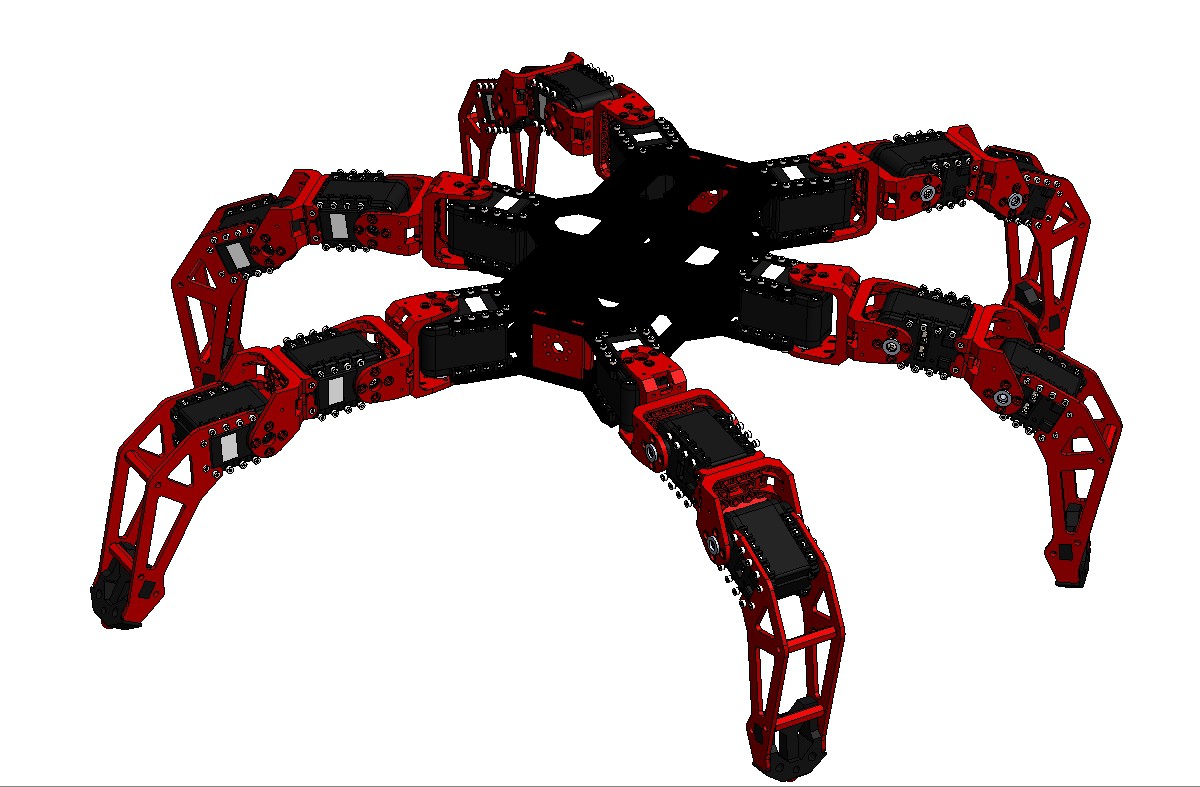
The legged robots are categorised depending on their leg types, leg orientations and joint configurations. Figure 2.1 shows the three hexapod models that are created in MapleSim. In light of the analysis given in the progress report, circular body-shaped model, shown in Figure 2.1-c was chosen for further development.
Figure 2.1 (a) Arachnid – Frontal, (b) Reptile – Frontal, (c) Reptile - Circular![]()
The structure of this report is organized as follows; in Chapter 2, a comparison between legged and wheeled robots is provided, in Chapter 3, the fundamental concepts associated with hexapod robots are given, following that, a hierarchical control architecture that may be divided as path planning and control is given in Chapter 4. Then, the simulation results that are obtained from MapleSim are presented in Chapter 5 and the report is concluded with future work and conclusion in Chapters 6 and 7, respectively.
2.1.Statements of Aims, Objectives, and Motivation
The aim of this project was to build a hexapod robot in the MapleSim simulation platform to test different path planning and control strategies for the hexapod robot. The steps that are taken to accomplish the aim are as follows:
- Circular and rectangular body-shaped hexapod robots are created in the MapleSim environment.
- Inverse kinematic equations are derived to coordinate the legged locomotion.
- 3 different biologically inspired walking gaits, tripod, ripple, and wave are implemented in the simulations.
- Static and dynamic stability analyses of the robot are undertaken.
- Dynamics of hexapod robot is examined and equations of motion are derived.
- Forces in each leg is calculated and a tilt control method is developed.
- A* path planning algorithm is used to find the body path that traverses from the start point to the target point.
- Probabilistic Roadmap Method (PRM) is implemented to step over obstacles within the workspace of the leg.
- Adaptive gait selector and zero moment point (ZMP) planners are implemented which improved the stability of the robot during locomotion.
- Inverse dynamics is implemented to improve the trajectory tracking of the robot legs.
2.1.Literature Review
Throughout the project, numerous resources have been studied and many different methods of implementation have been encountered and some of them are utilised to improve the project. This section is divided into 3 sub-sections which review the different legged robots, methods of path planning, and control strategies.
2.2.1. Legged Robots
As it was mentioned in the Introduction, one of the applications of legged-robots is demining; Nonami [2] and his colleagues designed the 4th generation of COMET, a hydraulically actuated hexapod robot, for land mine detection and demining. Figure 2.2–a shows a picture of COMET-IV which is powered by two 720cc gasoline motors, weighs 1500 kg and is capable of reaching a walking speed of 1 km/h [2]. COMET-IV uses force control for navigation on an uneven terrain. Figure 2.2–b shows ATHLETE which is a hybrid hexapod robot that is capable of both wheeled and legged locomotion [7]. It was developed by NASA for exploration of Mars [4]. It is capable of mapping an unknown environment, collecting samples with its scoop and gripper attachments, and transporting goods that weigh up to 450 kg [8].
![]()
Figure 2.2 Existing legged robots, adapted from [2] [4] [5] [6]
Roennau [5] demonstrated the 5th generation of LAURON which, unlike its ancestors, is designed with 4 degrees of freedom (DOF) in each of its 6 legs, giving it advantage to climb steeper surfaces. Figure 2.2–c shows LAURON V which was designed for search and rescue (SAR) missions [5]. RHex was develop by Boston Dynamics, what makes it special is its extraordinary design. RHex is a six-legged robot that has only 1 DOF at each leg [4]. RHex weighs about 12.5 kg and it is designed specifically for rough terrain [9]. It is capable of overcoming obstacle that is larger than its size and operate even if it is inverted [10]. Please, refer to the progress report for the other two products of Boston Dynamics, BigDog and LittleDog which are shown in Figure 2.2-d and Figure 2.2-f, respectively.
2.2.2.Path Planning
Rapidly exploring random tree (RRT) was first introduced by LaValle [11] which is a randomised path planning method that spreads in an omni-directional manner from both start and goal points until the two trees meet as it is shown in Figure 2.3–a. Belter and Skrzypczynski [12], made use of this method to obtain a collision-free trajectory over an object.![]()
Figure 2.3 Different path planning algorithms, adapted from [13] [14]
Figure 2.3–b shows Probabilistic Roadmap Method (PRM) which was used by Hauser [7] to find the shortest path between two points for a humanoid robot, HRP-2. This method is further explained in Section 4.2.1. Bai and Low [15] used artificial potential fields approach for path finding. An example of this method is shown in Figure 2.2–c where red cells represent the obstacles and grey intensity increases as the goal point is being approached. This algorithm is based on a gradient descent search method where the robot is treated as a point particle under the influence of a potential field [16]. The robot is attached to the goal point and it is repelled from the obstacles located within the environment [16].
2.2.3.Control
The operation of robot control architectures is based on a 3 step structure that consists of sensing, response, and action [4]. Figure 2.4–a shows the reactive control architecture, where an action is defined for different sensor readings. This method is used by the RHex robot which is shown in Figure 2.2-f. Although this architecture provides rapid speed of response the method is not suitable if predictive planned outcomes need to be produced [17]. Figure 2.4–b shows the structure of hierarchical control architecture which is used by Kolter [6] and Kalakrishnan [18] to control the LittleDog robot which successfully walks over uneven terrain. This architecture is more suitable for static environments where the goal is achieved in a planned manner [17]. However in the dynamic environments, the planning phase cause a slow response to changes [17].
![]() Figure 2.4 Robot control architectures
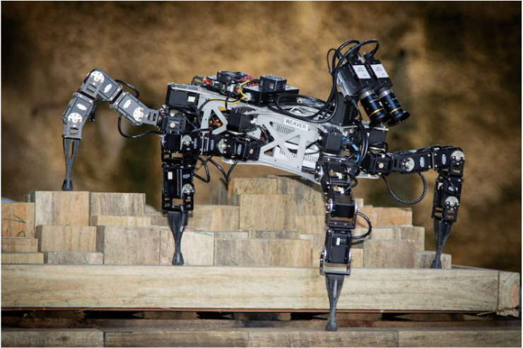
Figure 2.4 Robot control architecturesFigure 2.4–c shows the structure of hybrid control architecture where the two control architectures are combined to ameliorate the drawbacks of each architecture. The intermediate layer is required for a smooth transition between two architectures [17]. Bjelonic [19] and his colleagues implemented hybrid control architecture in hexapod robot Weaver which autonomously navigates on uneven terrain, shown in Figure 2.5.
![]() Figure 2.5 Weaver on the testbed.
Figure 2.5 Weaver on the testbed.2.3.Advantages of Hexapod over Wheeled Vehicles
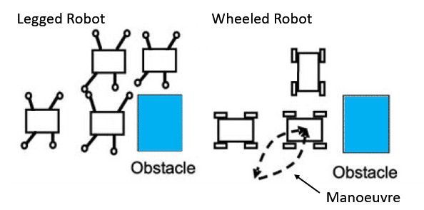
The legged robots have a number of advantages over the wheeled robots such as mobility and overcoming obstacles. Legged robots are omni-directional systems, i.e. it can change direction independently from its direction of motion whereas this is not the case for wheeled robots which require to manoeuvre in order to change direction. Figure 2.6 shows the difference of changing direction between the two types of robots, legged and wheeled robots. It can be seen that the legged robot moves side way to avoid the obstacle while the wheelled robot needs to manoeuvre.
![]()
Figure 2.6 Mobility comparison of legged and wheeled robots, adapted from [3]
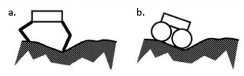
A legged robot is capable of maintaining its body level despite the changing slope of the surface that the robot is located on, as it is shown in Figure 2.7-a. In contrary, the body of a wheeled robot is always parallel to the slope of the surface, as it is shown in Figure 2.7-b.
![]()
Figure 2.7 Body tiltness correction of legged robots, adapted from [3]
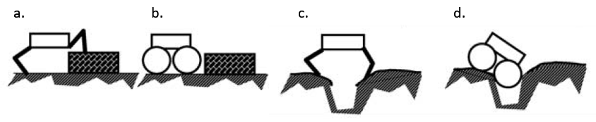
The legged robots are also more advantageous for tasks that require the robot to overcome obstacles and to operate on non-continuous terrain, since the legged robots are capable of stepping over an obstacle or a pit, shown in Figure 2.8-a and Figure 2.8-c, whereas a wheeled robot is simply stuck if the height of the obstacle is greater than the radius of its wheels, shown in Figure 2.8-b and Figure 2.8-d.
![]()
Figure 2.8 Overcoming obstacles advantage of legged robots, adapted from [3]
2.4.Disadvantages of Hexapod over Wheeled Vehicles
The legged robots are not commonly used due to the drawbacks associated with the complexity of the system, low locomotion speed, and high cost of manufacturing [3]. The legged robots are more complex in terms of mechanics and control, compared to the wheeled robots, e.g. the hexapod robot has 3 degrees of freedom (DOF) at each leg, and a total of 18-DOF whereas a 4-wheeled robot has only 2-DOF, i.e. 2 wheels for traction and steering, and 2 passive wheels [3]. In addition, a hexapod robot coordinates the motion of all 18 joints simultaneously, in order to navigate from point A to point B.
Another disadvantage of legged robots is the low locomotion speed since neither the statically stable nor the dynamically stable hexapod robots move as fast as the wheeled robots [3]. Moreover, due to the increased complexity, the legged robots require more actuators, motor drivers, and sensors, therefore the cost of manufacturing a legged robot is significantly over a wheeled robot. The Table 1-1 shows the quantity of needed components which are provided for the comparison and cost estimation purposes.
![]()
Table 1‑1 [3] Estimated figures which indicate the cost and complexity comparison
-
1. Abstract
06/29/2017 at 14:32 • 0 commentsAs a result of exponentially developing science and technology, tremendous amount of research is being undertaken on mobile robots which are commonly used in both domestic and industrial applications. Hexapod robot is a type of legged mobile robot that is autonomous and omni-directional.
This report presents the hierarchical control architecture that is developed to control a six-legged robot which was modelled within the MapleSim environment. In addition, 2 different map-based path planning algorithms, A* (star) and Probabilistic Roadmap Method (PRM) are implemented to find the shortest path to a given goal and to step over obstacles, respectively. Static and dynamic analyses of the hexapod model are given and an adaptive gait selector which was implemented to improve the stability depending on the terrain slope, is presented. A geometric approach to tilt control has been developed and implemented. Moreover, a multivariable control was implemented in the low level controller of the hierarchy for position control and trajectory tracking. MATLAB and MapleSim are widely used throughout the project and the important codes are provided in the Appendix.
The obtained results show that the hexapod robot successfully navigates between point A and point B in both of the implemented approaches: slalom and pedestrian-lane-change.
Key words: Hexapod, MapleSim, Hierarchical Control, Path Planning
-
3D Design
05/30/2017 at 22:43 • 0 comments![]()
Hexapod Modelling, Path Planning and Control
My Final Year Dissertation Project - Awarded with a First Class Degree
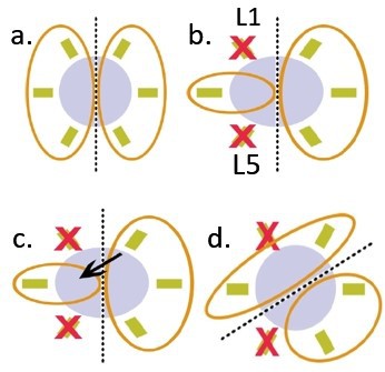
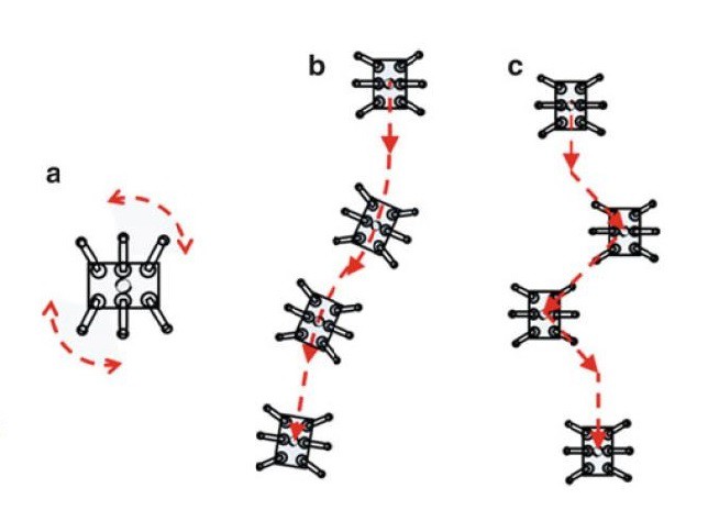

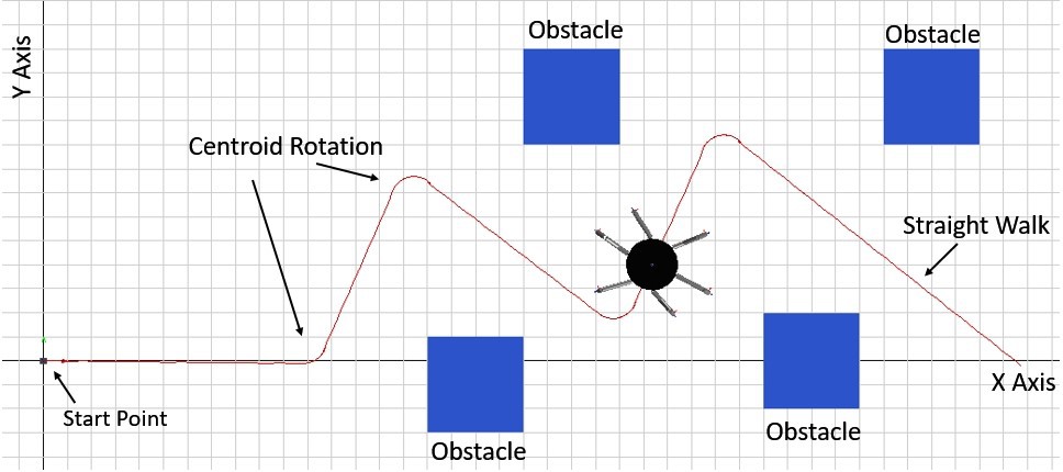
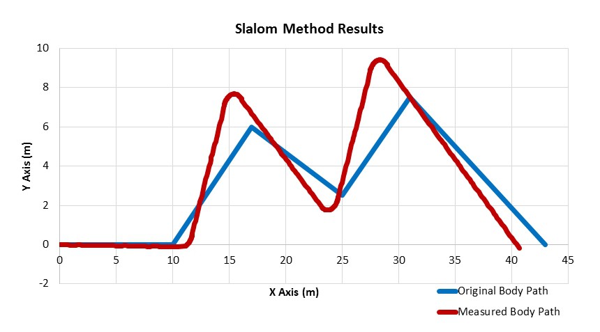
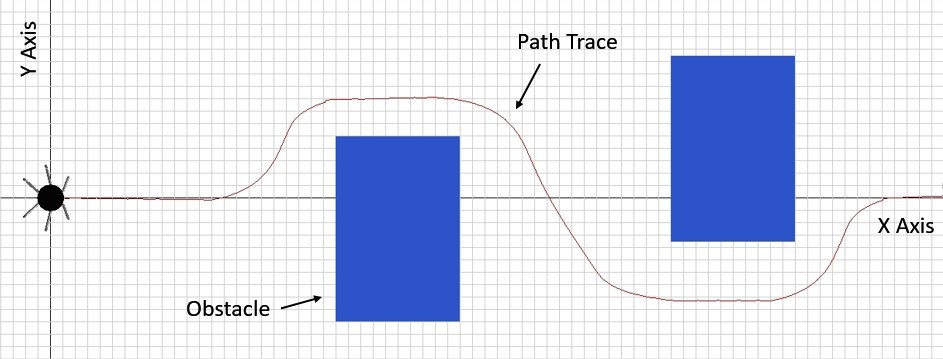
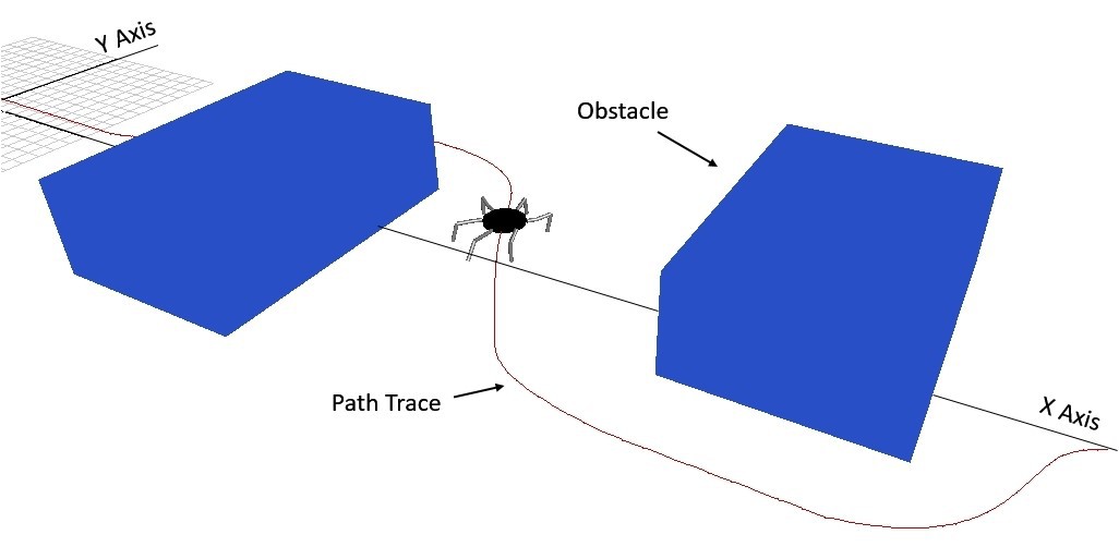
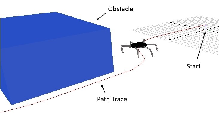

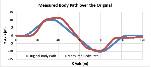
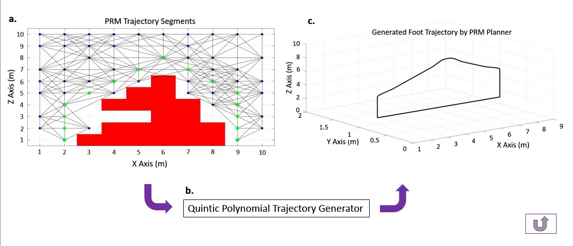
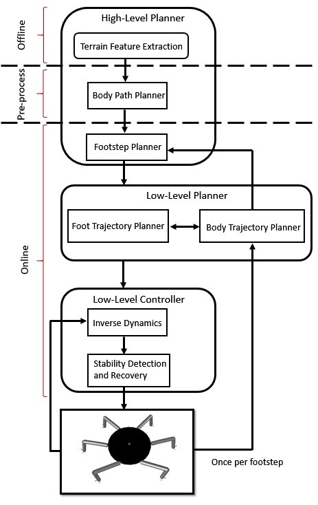
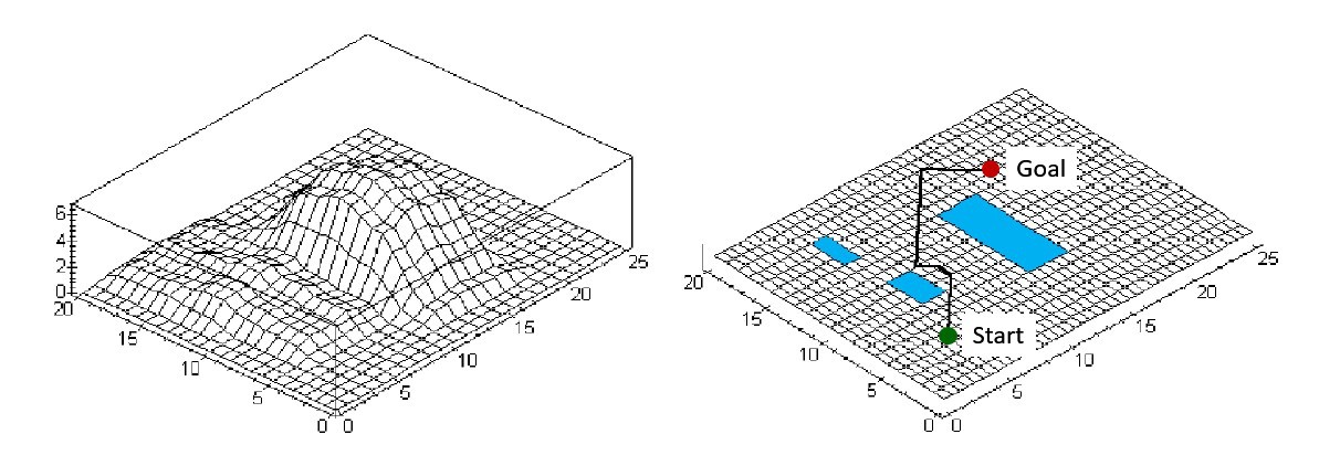 Figure 4.2-a Uneven terrain and the 2D representation of terrain, adapted from [15]
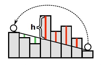 Figure 4.3 Collision map of a foot trajectory over an obstacle, adapted from [28]
 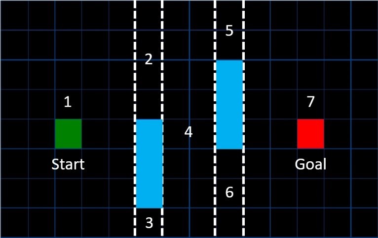 Figure 4.4 Occupancy Grid Representation
 Figure 4.5 Adjacency Map of the Occupancy Grid.
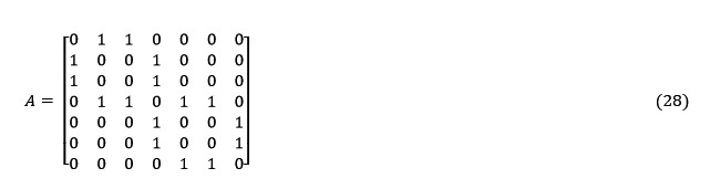 A* (star) path planning algorithm determines the cost of the 8 surrounding nodes by using Equation 28,
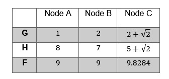 Table 3‑1 Example G, H, and F values of Nodes A, B, and C.
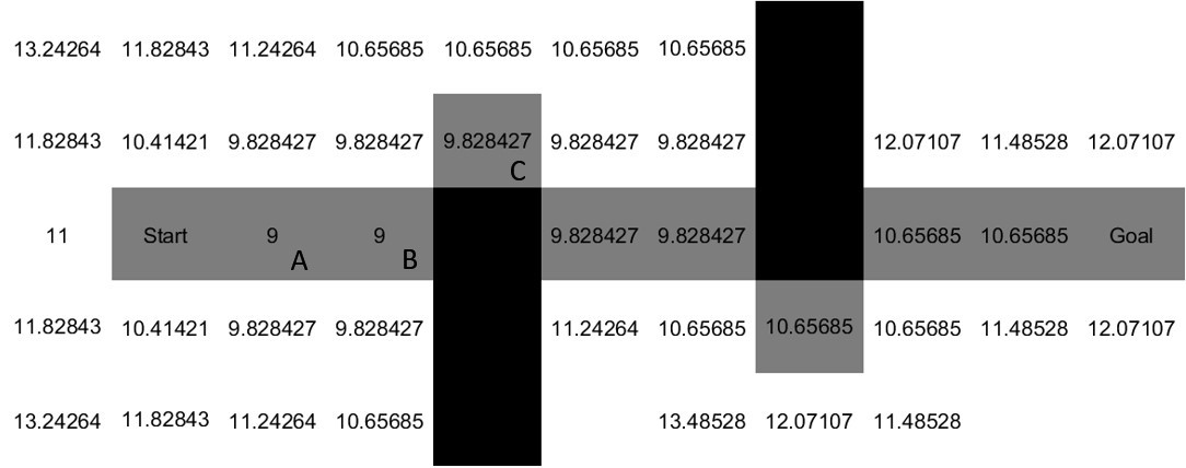 Figure 4.6 The body path found by the A* algorithm MATLAB Script 8-3 (in Appendix) was used to generate the path in Figure 4.6 which shows the generated body path between Start node and Goal node in grey and the obstacles are shown in black. It can be seen that, the path given in Figure 4.6 is not smooth. In order to obtain a smoother body path, a 2nd order low pass Butterworth filter is applied and hence, the body path given in Figure 4.7 is generated. This path has been used in the MapleSim simulations as the test body path.
 Figure 4.7 The body path that is used in the MapleSim simulations
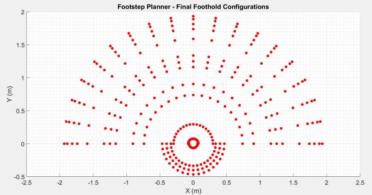 Figure 4.8 X-Y View of the possible Final Foothold Configurations.
 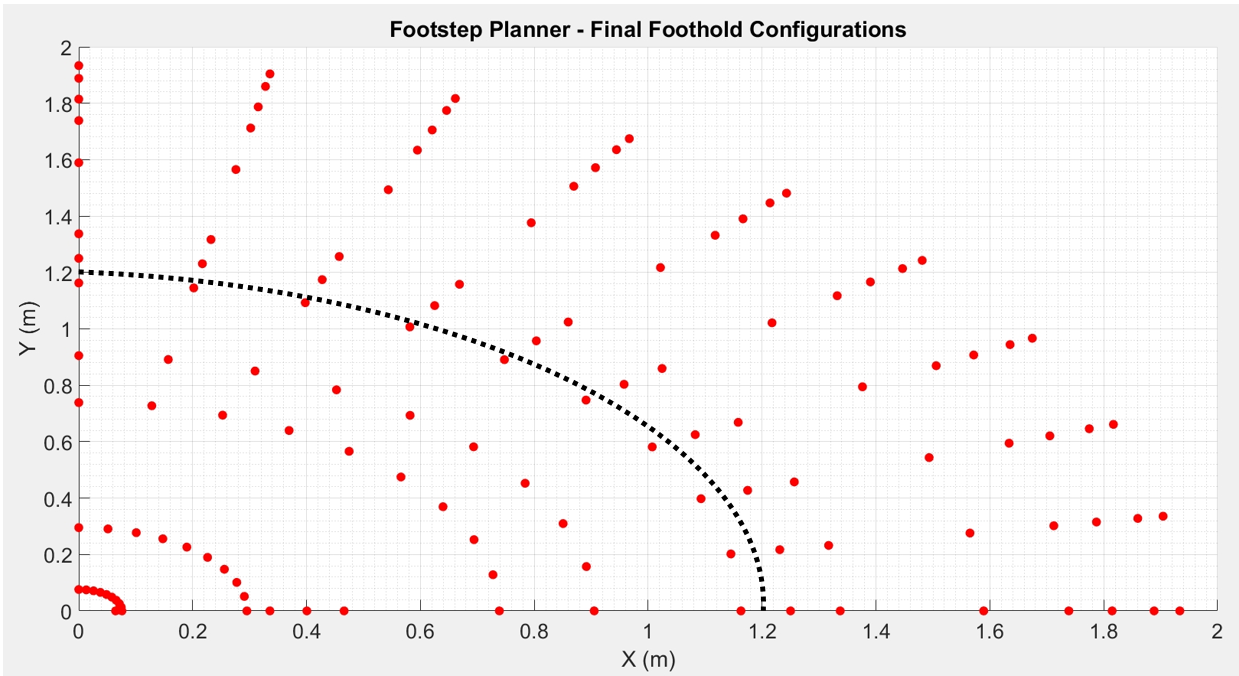 Figure 4.9 X-Y View of the possible Final Foothold Configurations in the 1st Quadrant.
 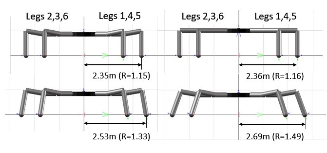 Figure 4.10 Different leg configurations and corresponding R values of the MapleSim Model.
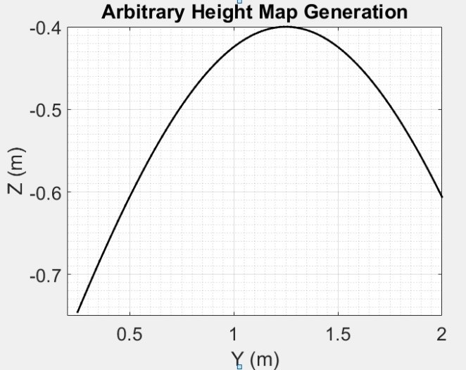 Figure 4.11 Curve that was used to generate the uneven terrain
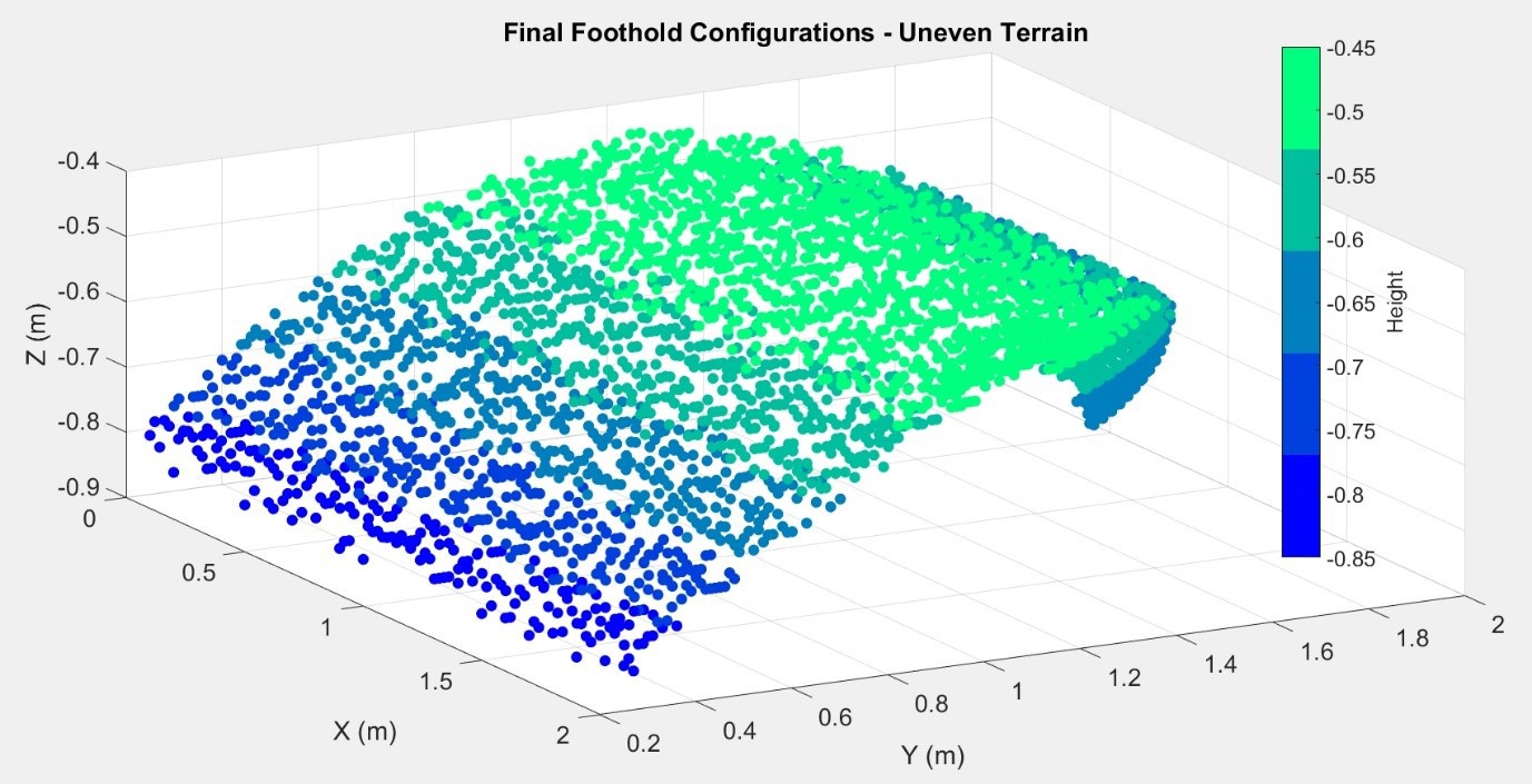
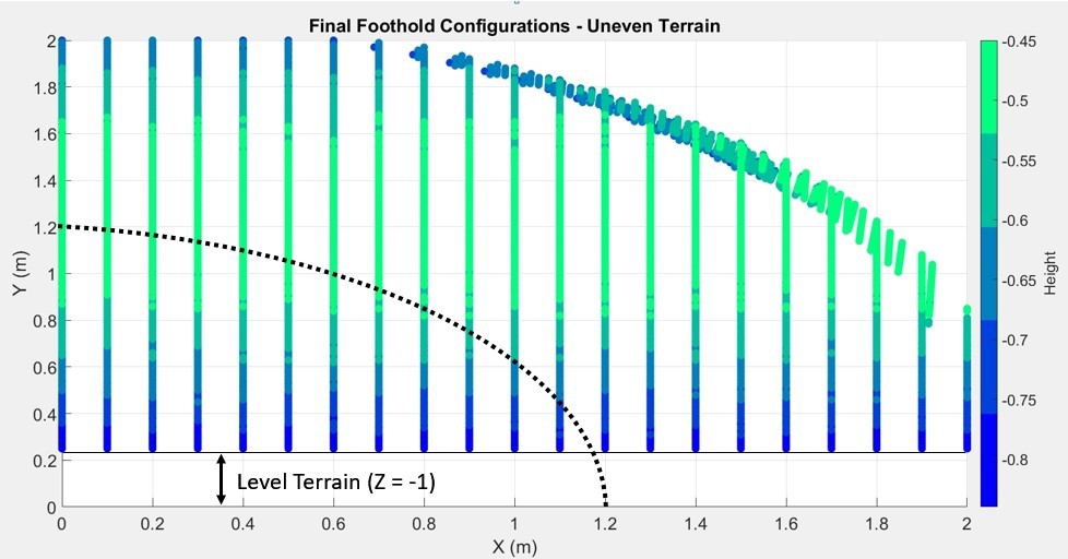 Figure 4.13 X-Y view of the final foothold configurations on an uneven terrain
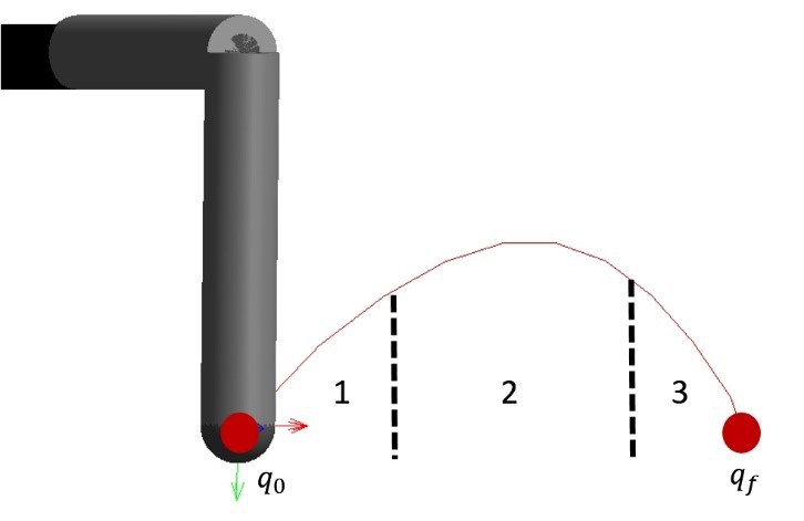 Figure 4.14 Foot Trajectory between initial and final configurations.
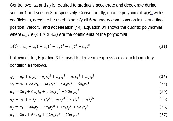
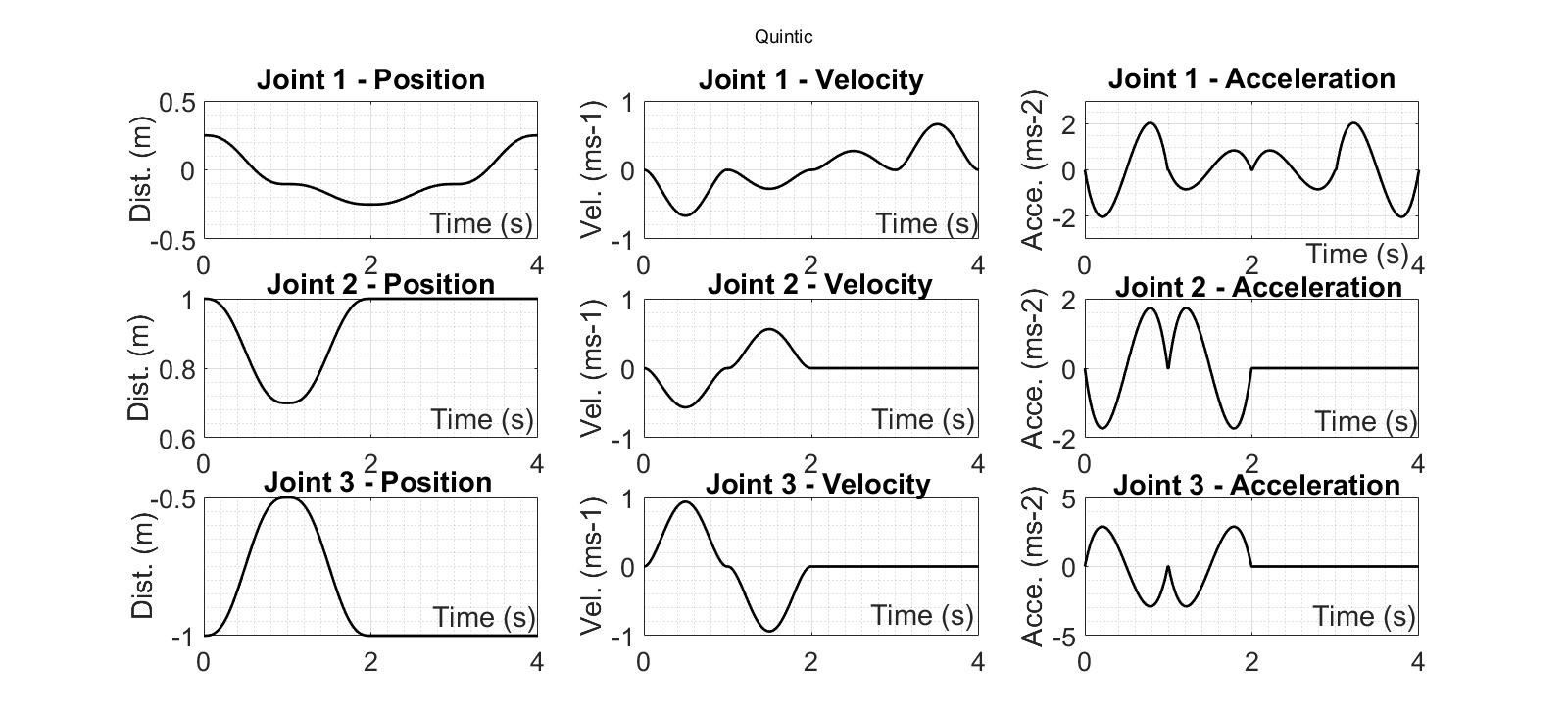

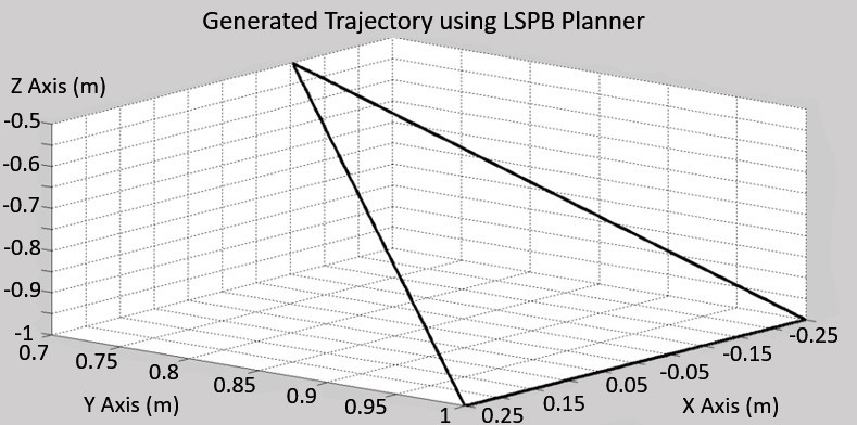 Figure 4.17 The Foot Trajectory generated using the LSPB Planner
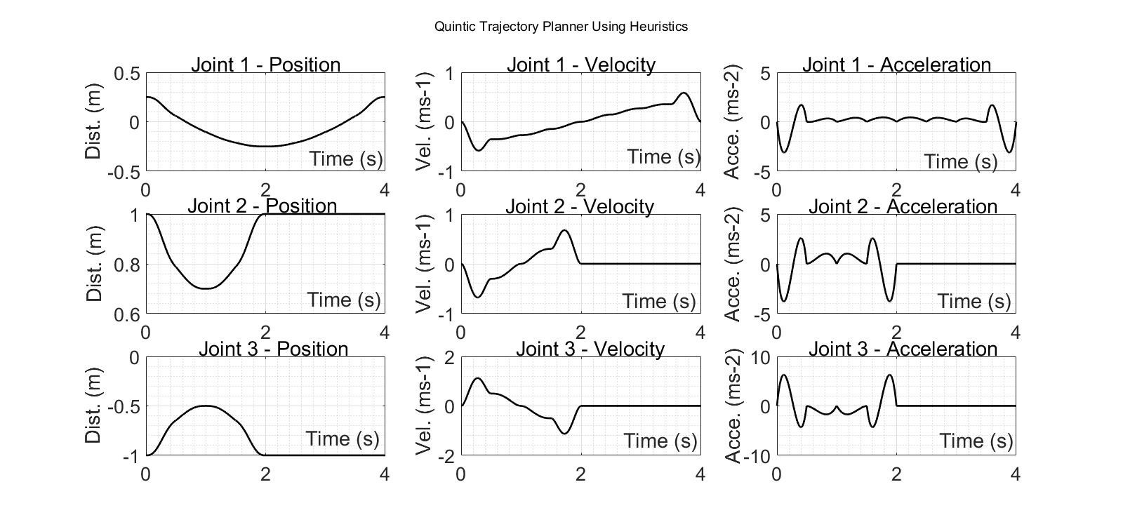 Figure 4.18 Position, velocity, and acceleration calculated using heuristics
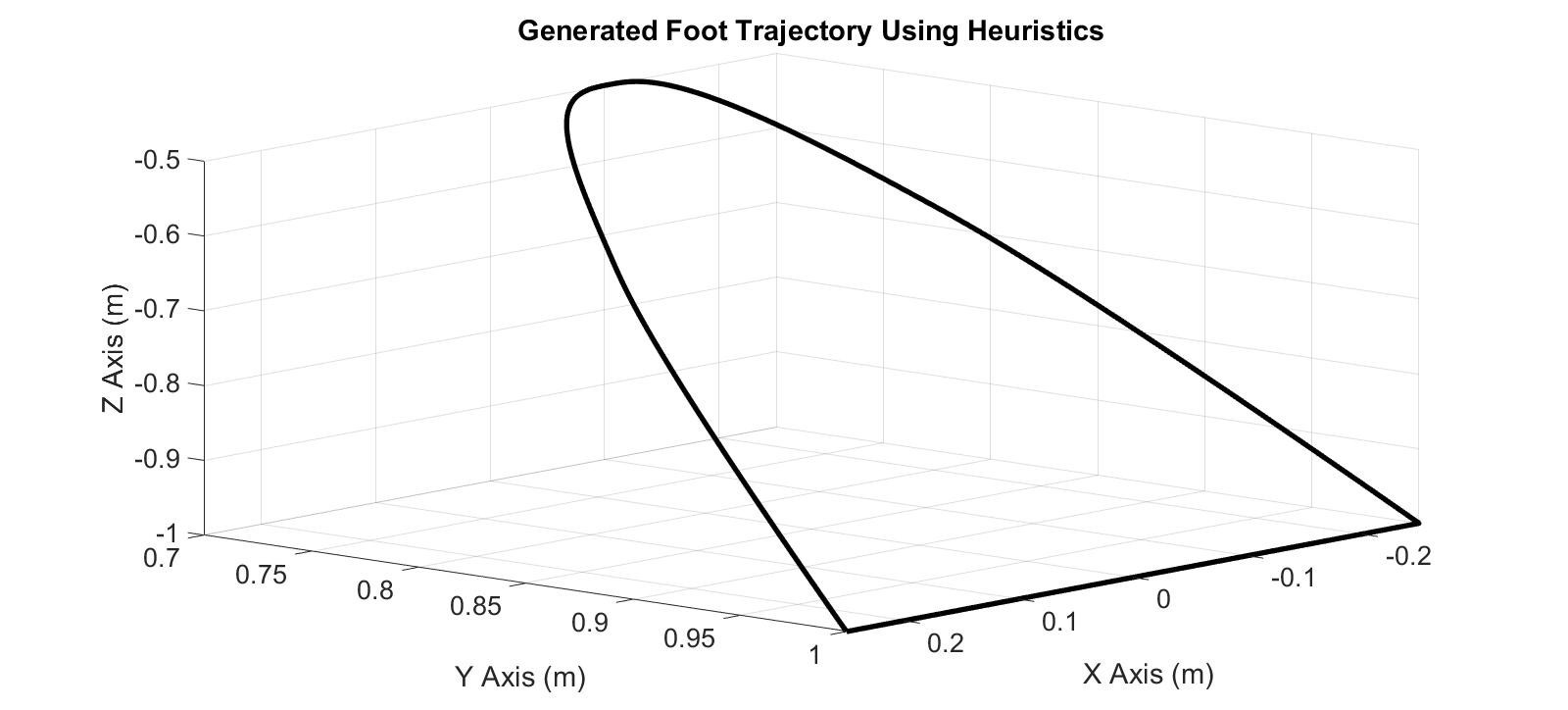 Figure 4.19 The Foot Trajectory generated using heuristics
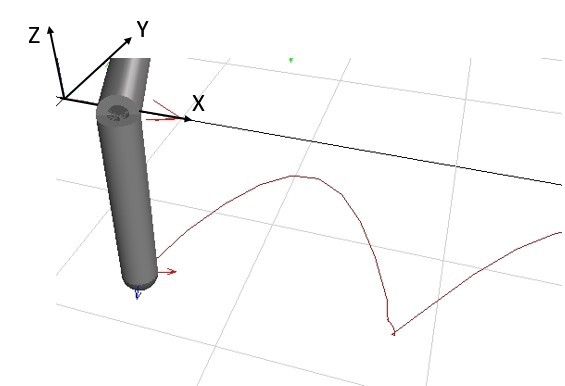 Figure 4.20 MapleSim implementation of the generated trajectory
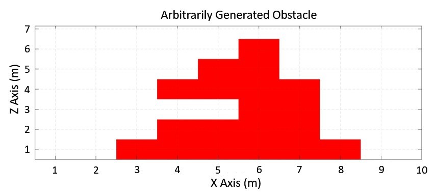 Figure 4.21 Arbitrarily generated obstacle to test the PRM algorithm
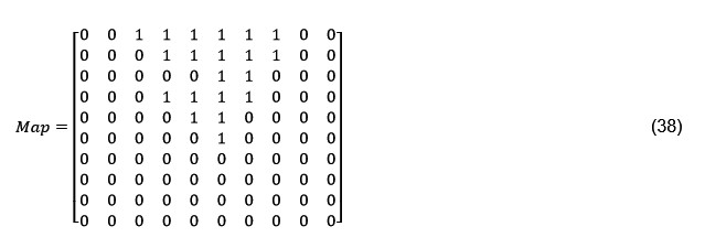 The chosen path planner algorithm, PRM, generates a set of random configurations within Q then the end effector configurations that lie within Qobs are neglected and the configurations that are located within the borders of the Qfree are connected by straight lines to form pairs of configurations given that the lines do not violate the Qobs [16]. The lines that introduce a collision, i.e. violate the Qobs are also neglected. Then, the Cartesian coordinates of the configurations that are located on the shortest roadmap connecting the qo and qf are used by the trajectory planner to generate the collision free foot trajectory that lands on the position projected by the footstep planner. Figure 4.22 shows the set of configurations that needs to be followed to prevent a collision with the arbitrarily generated obstacle, where the randomly chosen configurations are denoted by blue nodes and the configurations that lie on the shortest roadmap are denoted by green nodes. In this particular example, the qo and qf are chosen as (2,1) and (9,1), respectively, whereas in the simulation the initial and final configurations are provided by the footstep planner.
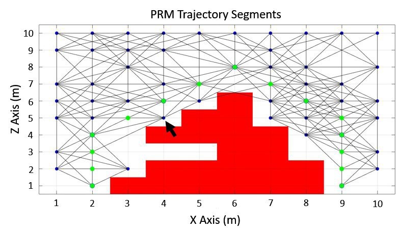 Figure 4.22 The intermediate end effector positions that connect qo and qf.
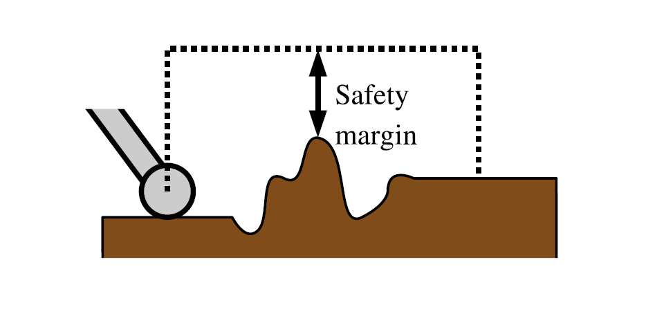
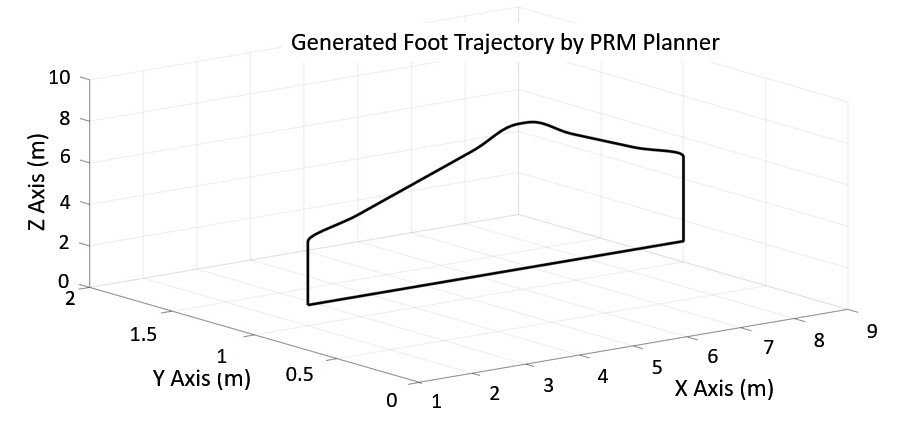

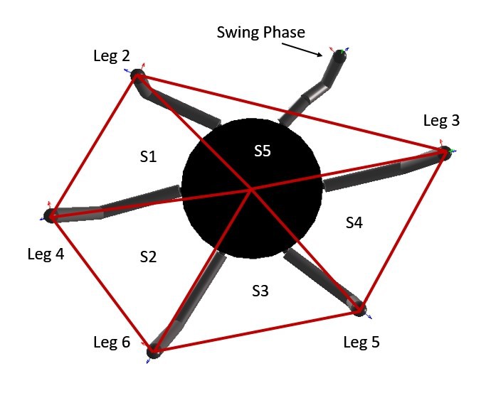
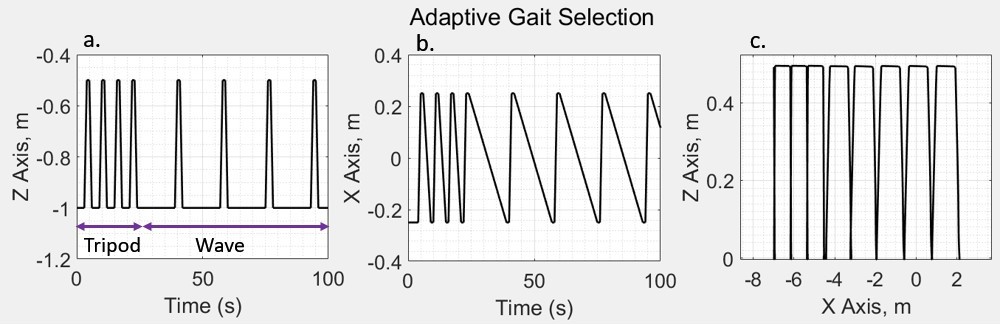
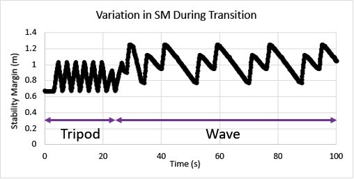
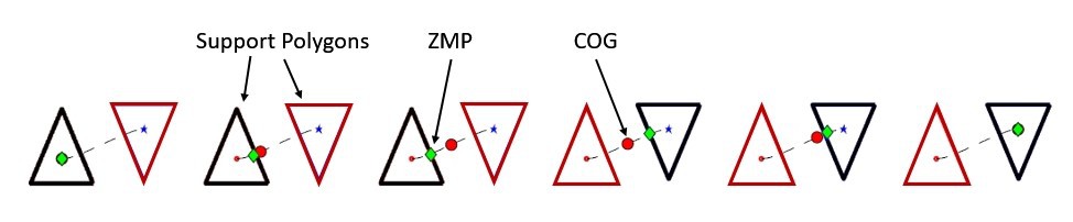 Figure 4.29 The trajectory of COG and ZMP during tripod gait, adapted from [18]
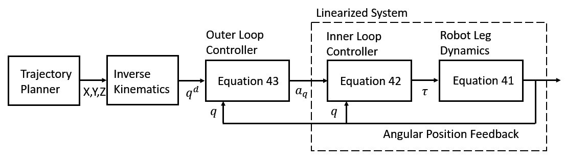 Figure 4.30: Inner Loop – Outer Loop Linearized Control, adapted from [16]
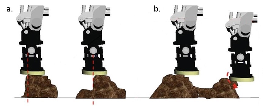
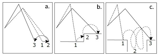
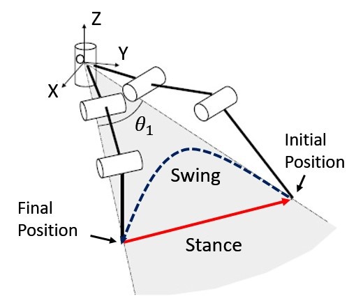
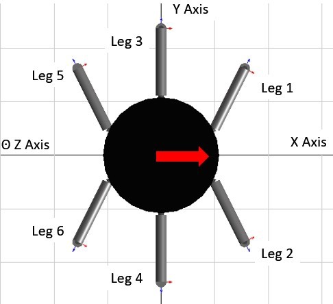
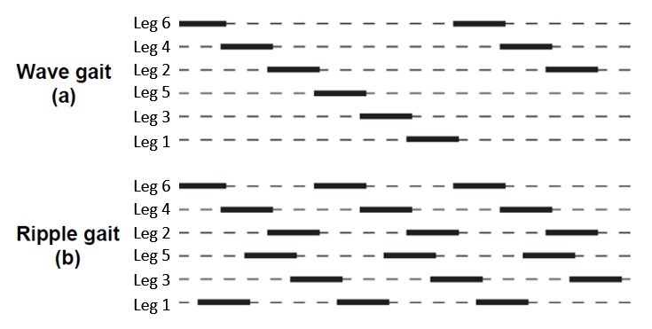
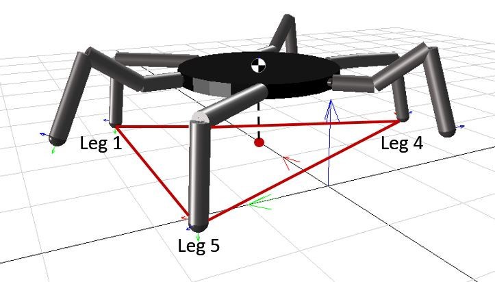
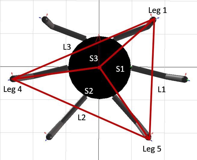

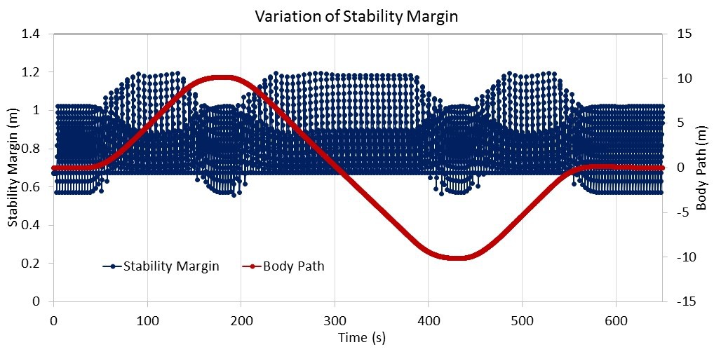
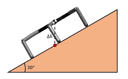
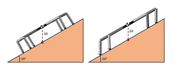
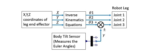
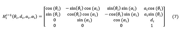
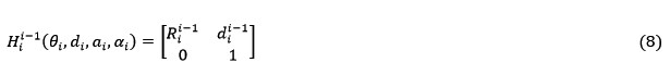
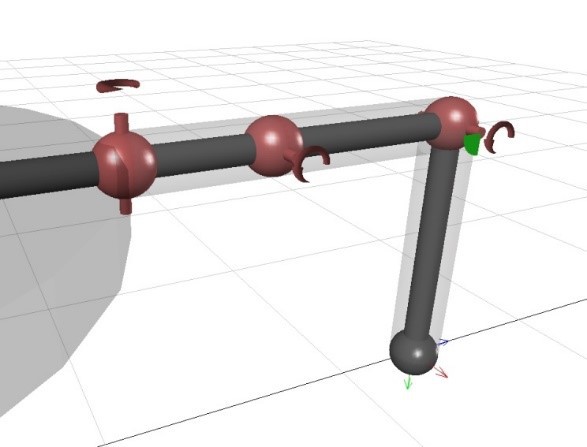
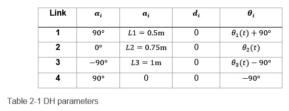
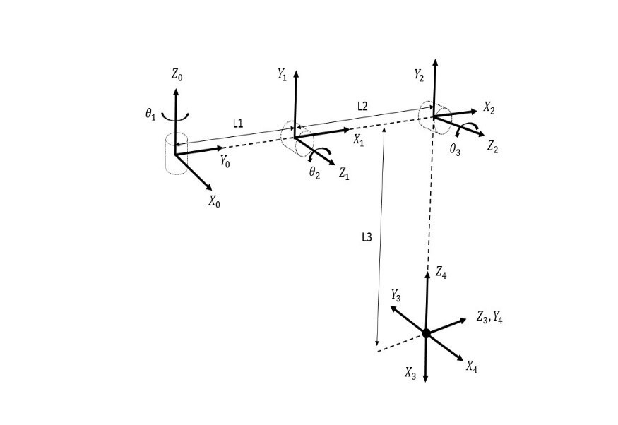 Figure 3.12 Forward kinematic model of the robot leg
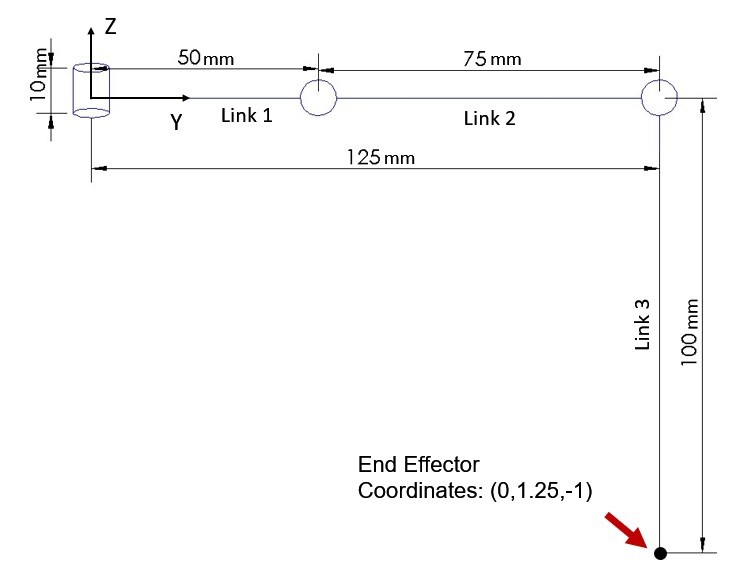
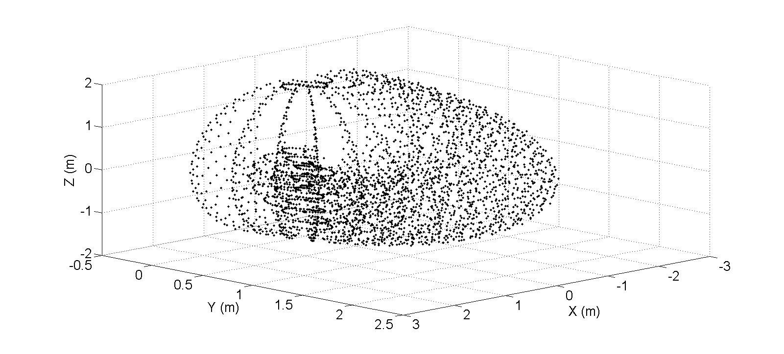
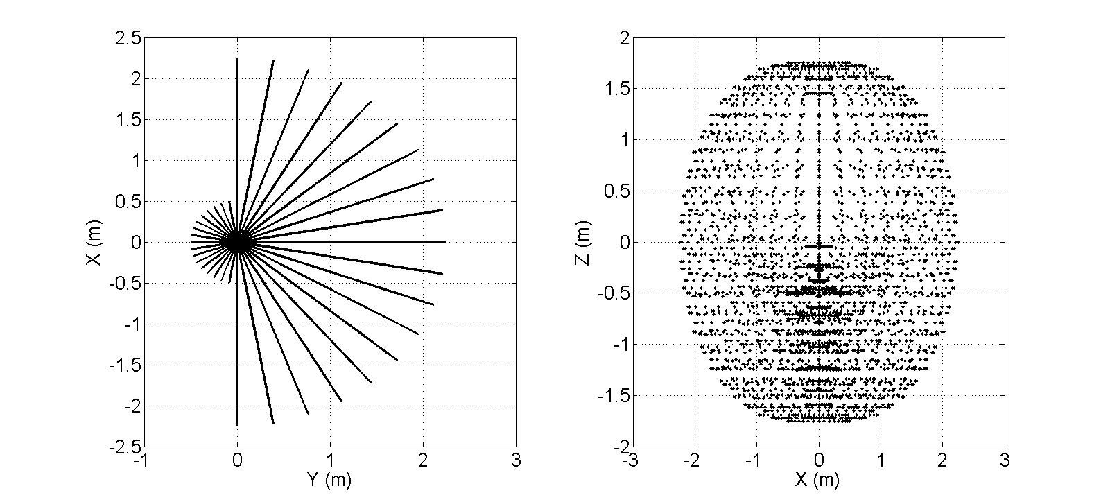
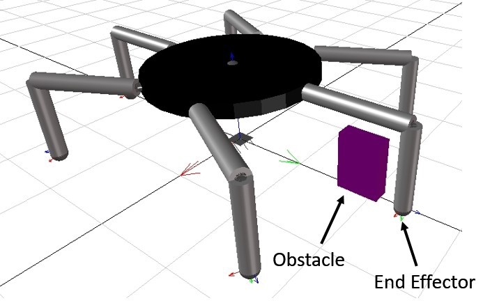
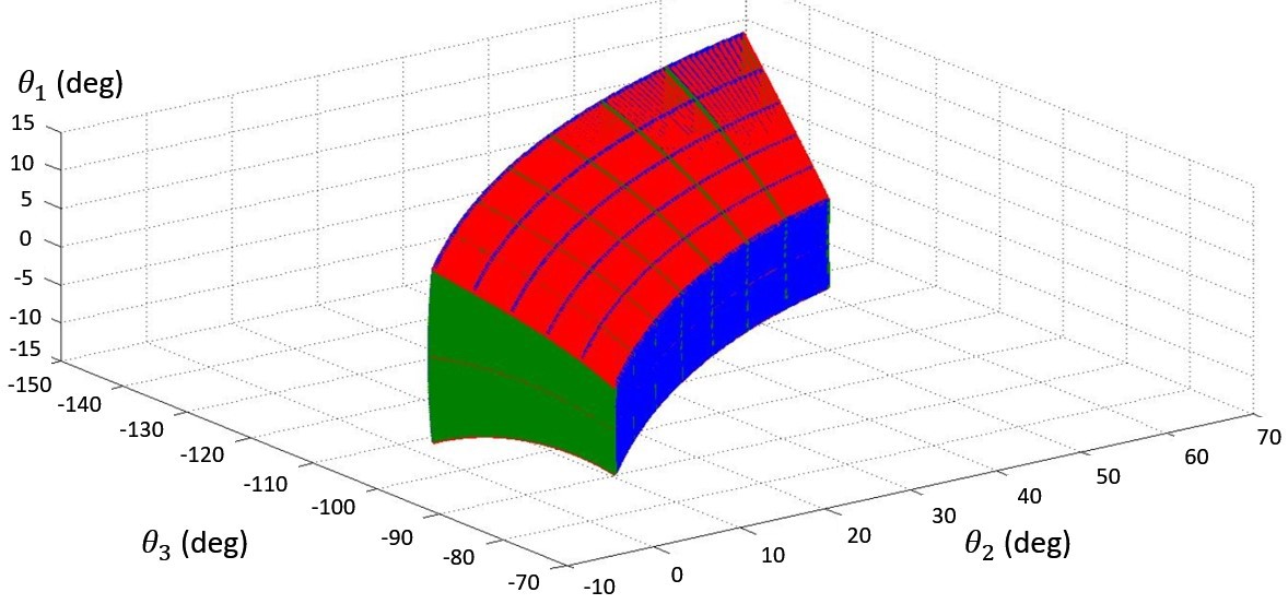
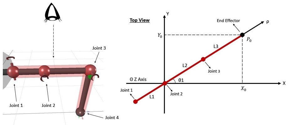
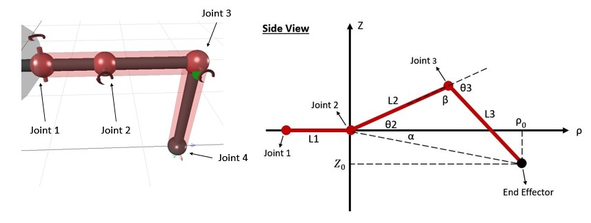
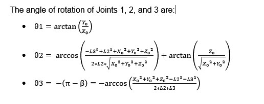
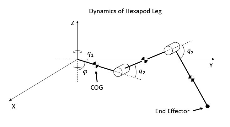
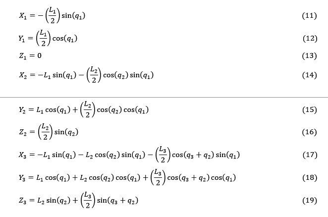
 Figure 3.19 Caartesian coordinates of COG of links 1, 2, and 3
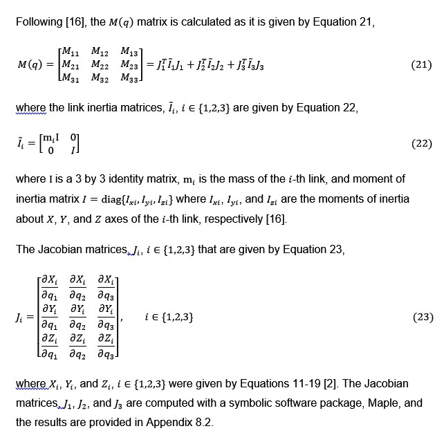
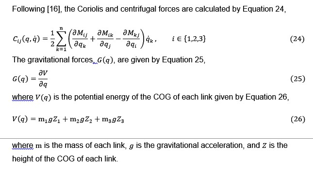
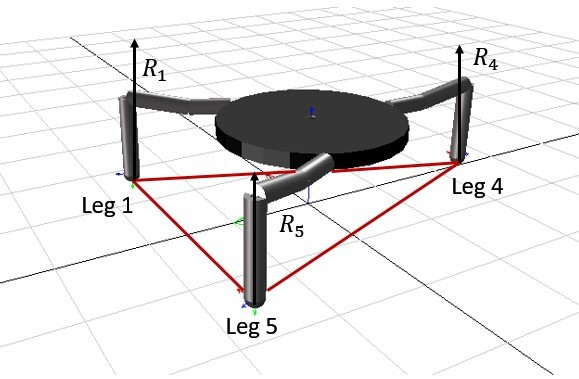
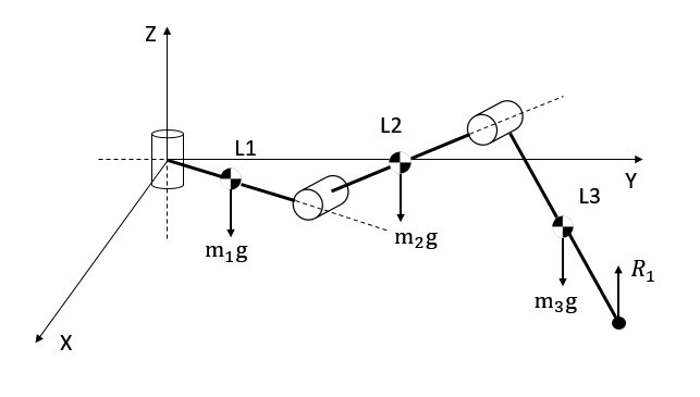
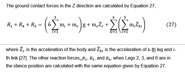
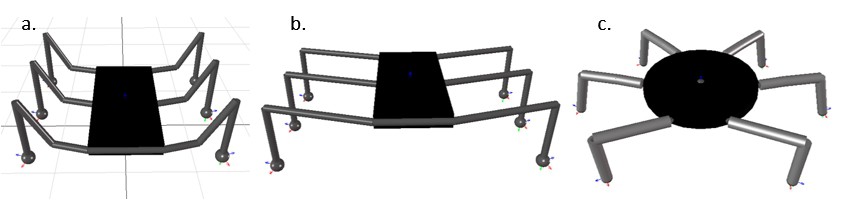
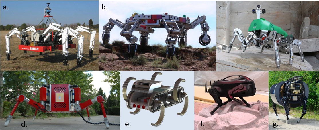
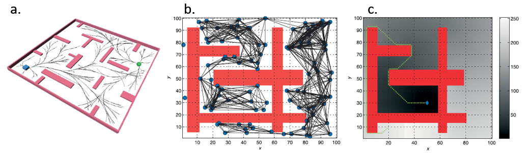
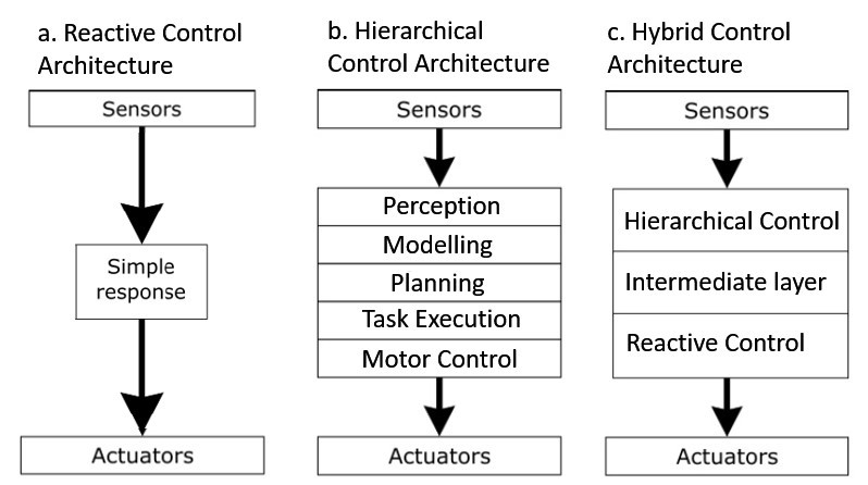 Figure 2.4 Robot control architectures