Jean-François Duval
-
September 2015 Project Update - Semifinals
09/18/2015 at 14:21 • 0 commentsHello Hackers!
In the same spirit as my quarter-finals project update, here’s one post containing all the information for the next judging round. Please excuse the repetitions!
- Video: FlexSEA - Hackaday Prize Semifinals (that's the one embedded above)
- Video: Prof. Hugh Herr talking about the FlexSEA project
- You can get a copy of the software projects and the hardware design files.
- In terms of system design document, please refer to my thesis. It contains extensive details about the hardware and the software. It's a great snapshot of the design as of May 2015.
- For more detailed design descriptions, consult the numerous Project Logs that I wrote about critical aspects of the project.
- As far as licensing goes, the thesis is licensed under Creative Common Attribution-NonCommercial-ShareAlike (CC BY-NC-SA 2015) and the hardware files are Open Source Hardware. Drop me a line if you use them, I’m curious to know about your projects.
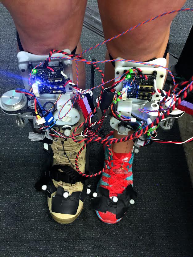
- Last time I linked to a short video shot by my colleague and friend Luke testing a strain-gauged based force controller on FlexSEA-Execute 0.1 for his exoskeleton. Much more exciting, here’s a video of him walking with one of his exoskeleton prototypes! You can also see his latest work in my Semifinals video.
- I started working on the next hardware revision, FlexSEA-Execute 0.2. All the details are in Working toward FlexSEA-Execute 0.2. The wide-input range power supply (18-50V in, 10V out, 82%+ efficiency) PCB is being manufactured right now, and a good part of the gate driver test board is designed. Exciting times!
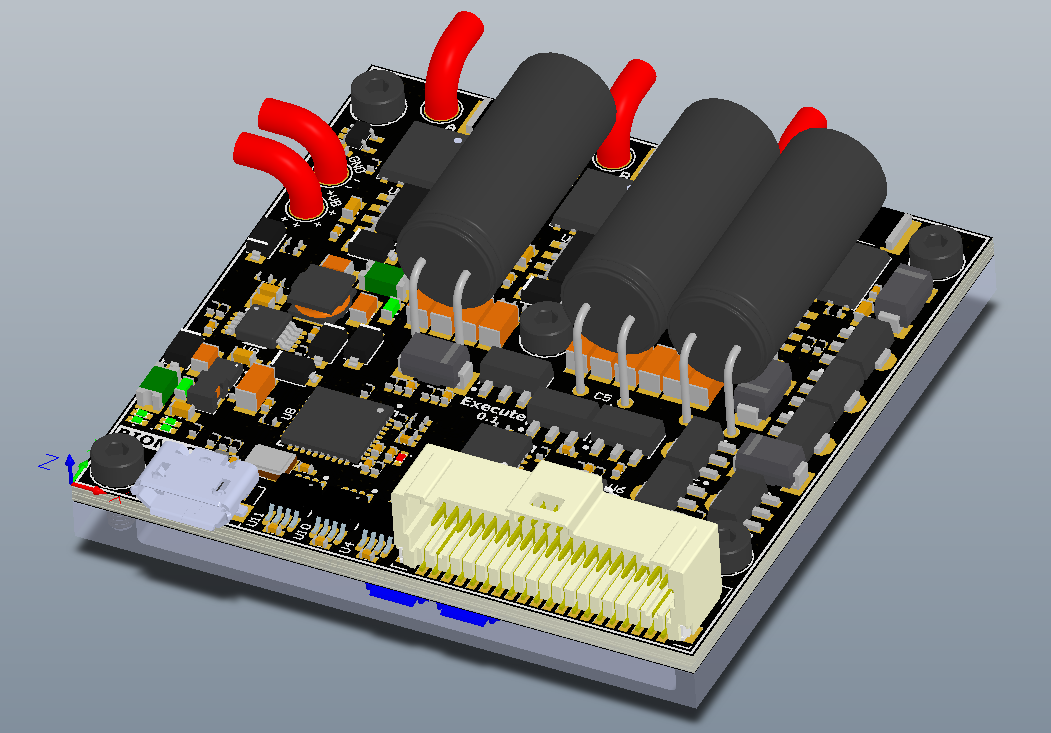
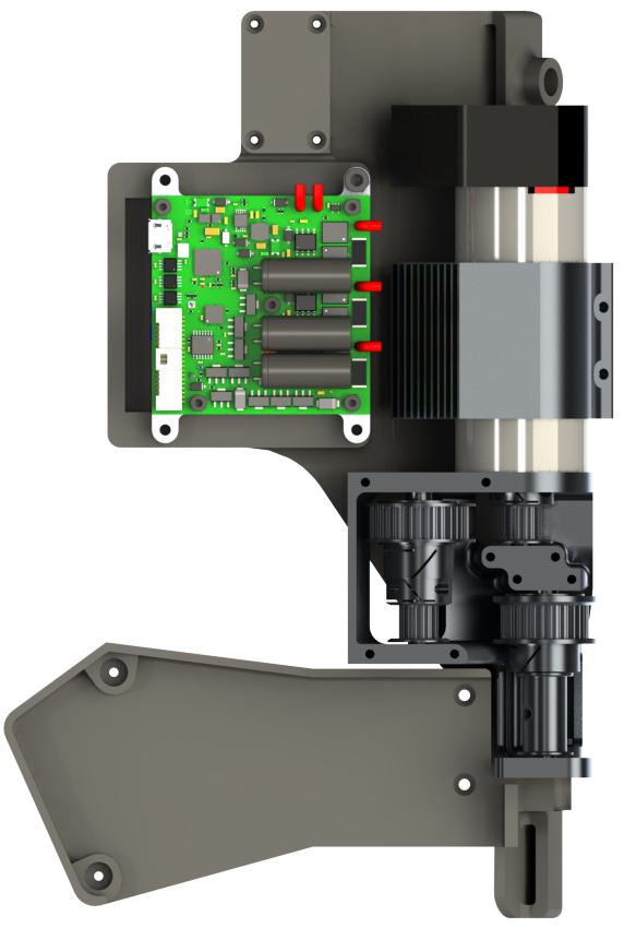
- One of the requirements is “artist’s rendition of the “productized” design/look and feel of the project”… Does beautiful layout and 3D CAD qualifies as art? I bet it does. In The evolution of FlexSEA prototypes I show pictures of the 3D design, and below you’ll see a screenshot of Execute integrated in the ExoBoot.
- Do not hesitate to ask me questions about the system in the comments below!
- I'm looking for contributors for the project. Drop me a line if you are interested.
![]()
-
So, why am I spending all this time describing technical aspects of the project?
09/17/2015 at 19:58 • 0 commentsI started playing with electricity and motors when I was a kid and I spent countless hours trying to build DIY RC cars and robots as a young teenager, without any real success. Keep in mind that this was before the age of the Arduino, when programming a PIC16F84 in ASM was the way to go. And that was hard. I still remember the amazing feeling from when I first got a RF remote control working, in C, on an 18F452-centered custom circuit and PCB! Years later, with an Electrical Engineering degree and a Master of Science in my pocket, I did not forget my roots. I’m using this project page as a teaching tool to help you in your projects. I’m covering technical implementation that are typically hard for hobbyists, and hopefully I’m finding the right words and examples to make it more accessible. I’m trying to make the world a better place with FlexSEA, but also by making a complete engineering design freely available to the public, with detailed explanations. What would you like to know? Ask in the comments!
-
Controlling a brushless motor (BLDC): Software
09/07/2015 at 19:45 • 0 commentsAs a starting point, I highly recommend reading AN857 Brushless DC Motor Control Made Easy & AN885 Brushless DC (BLDC) Motor Fundamentals from Microchip. The So, Which PWM Technique is Best? series from TI will then complement your knowledge of BLDC commutation.
===
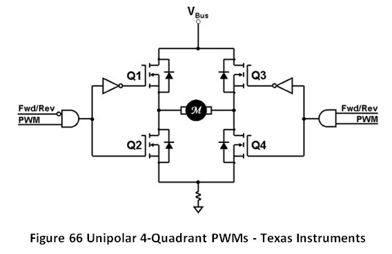
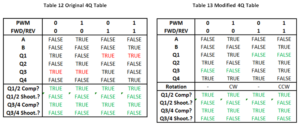
A four quadrant PWM commutation table is required to support bidirectional motor control with regenerative currents. Figure 66 is part of “So, Which PWM Technique is Best?” by Texas Instrument.
![]()
Table 12 was created from Figure 66. ‘A’ and ‘B’ are the intermediary signals, at the output of the AND gates. The red text indicate a problem: this table sets steady-state high values on the high-side MOSFETs. The gate drivers used on FlexSEA-Execute can’t support this. The two NOT gates were moved from the high-side to the low-side to fix this problem, as presented in Table 13. A test was made to confirm that the half-bridges are using complementary switching and that they are never ON at the same time (shoot-through).
![]()
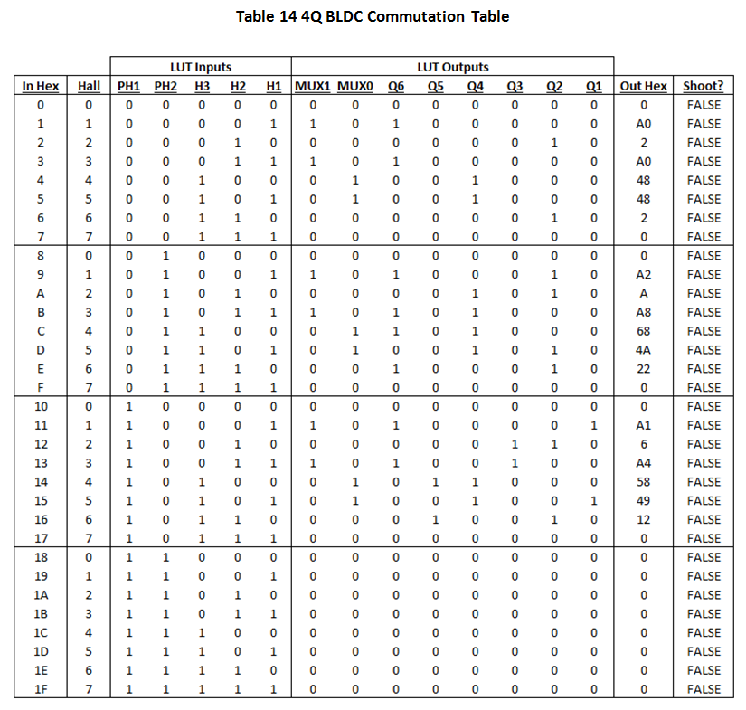
This table has to be expanded for three phase brushless motors. The order of the phases is determined by the Hall Effect sensors present in most research-grade brushless motors, such as the Maxon EC-30 used in this experiment. The PSoC 5LP look-up table (LUT) component supports a maximum of 5 inputs and 8 outputs. The 3 Hall sensors and the 2 PWM phases use all the inputs; the Direction signal (to change from clockwise to counter-clockwise rotation) cannot be integrated in the table. Table 14 shows the relation between the input signals and the output signals. MUX0 and MUX1 are used for the analog multiplexer that controls the current sampling.
![]()
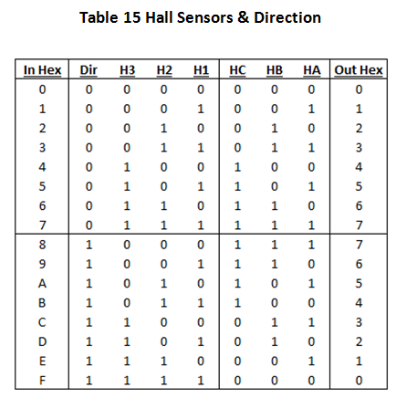
Table 15 presents a second LUT, used to control the direction of the rotation.
![]()
Of course, no one likes big look-up table in PNG format, so here’s the Excel sheet I used. The complete system can be seen in Figure 67.
![]()
The look-up table is registered with the PWM edge to avoid transitions from happening in the middle of a PWM cycle, when the Hall code is changed; in such an event the dead-time would not apply. The 6 PWM outputs were connected to a logic analyzer while the motor was spinning to confirm the validity of the table:
![]()
In terms of code, here's the function that gets called by all the other motor control functions:
//Controls motor PWM duty cycle
//Sign of 'pwm_duty' determines rotation direction
void motor_open_speed_1(int16 pwm_duty)
{
	int16 pdc = 0;

	//Clip PWM to valid range
	if(pwm_duty >= MAX_PWM)
		pdc = MAX_PWM;
	else if(pwm_duty <= MIN_PWM)
		pdc = MIN_PWM;
	else
		pdc = pwm_duty;

	//Save value to structure:
	ctrl.pwm = pdc;

	//Change direction according to sign
	if(pdc < 0)
	{
		pdc = -pdc;	//Make it positive
		MotorDirection_Write(0);
	}
	else
	{
		MotorDirection_Write(1);
	}

	//Write duty cycle to PWM module
	pdc = PWM1DC(pdc);
	PWM_1_WriteCompare1(pdc);
	PWM_1_WriteCompare2(PWM2DC(pdc));	//Can't be 0 or the ADC won't trigger
}
And here's an extract of the .h file://PWM limits #define MAX_PWM 760 //760 is 96% of 800 #define MIN_PWM -MAX_PWM #define DEADTIME 55 //Make sure that it matched the hardwar e setting! #define PWM1DC(pwm1) MAX(pwm1, DEADTIME) #define PWM2DC(pwm1) MAX(((pwm1 - DEADTIME)>>1), 10)And that’s it! You now have a complete reference for sensored brushless DC (BLDC) commutation on a PSoC 5, with a 4Q table. -
Controlling a brushless motor (BLDC): Hardware
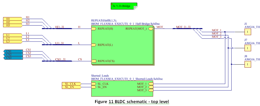
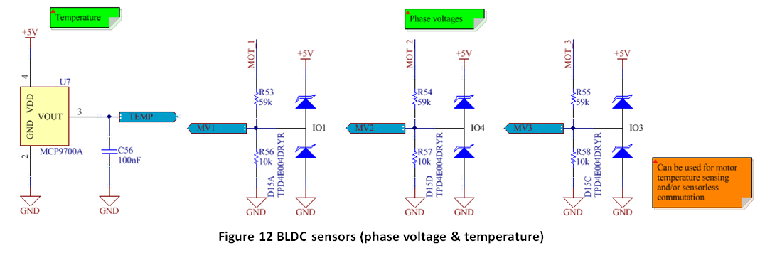
09/07/2015 at 19:18 • 0 commentsThe BLDC schematic consists of 3 copies of the Half-bridge sheet (motor commutation), the Shorted-Leads protection circuit, phase voltage sensing and bridge temperature sensing.
![]()
![]()
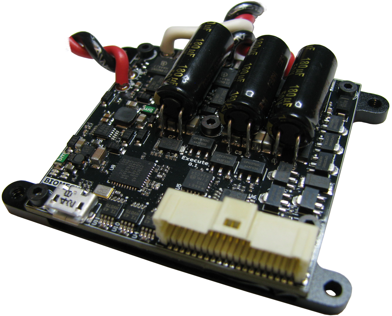
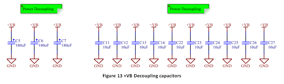
U7 (temperature sensor) is routed close to the power MOSFETs. Figure 13 shows the decoupling capacitors present on the Power Supply schematic sheet. They are mainly used for the BLDC driver. C11-14 & C22-27 are relatively small ceramic capacitors. Their total value, 100µF, is not sufficient to guarantee that the bus voltage won’t exceed the limits if a large amount of regeneration is done. C5 to C7 are used to absorb all this energy (and to provide power during switching transitions as well), but they are bulky. In applications were volume is highly constrained, C5-7 can be removed if an external protection circuit is added to the system (typically, a bus-dump semiconductor or resistor). This should be done with care.
Half-bridges![]()
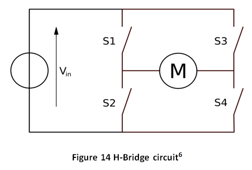
![]() DC motors are commonly driven by a circuit called an H-Bridge. An H bridge is an electronic circuit that enables a voltage to be applied across a load in either direction. Closing S1 and S4 will make the motor turn in one direction, while closing S2 and S3 will make it rotate in the opposite direction. Closing S1 and S3, or S2 and S4, can be used to brake the motor. Closing S1 and S2, or S3 and S4, will create a short circuit on the power supply and can lead to catastrophic failure.
DC motors are commonly driven by a circuit called an H-Bridge. An H bridge is an electronic circuit that enables a voltage to be applied across a load in either direction. Closing S1 and S4 will make the motor turn in one direction, while closing S2 and S3 will make it rotate in the opposite direction. Closing S1 and S3, or S2 and S4, can be used to brake the motor. Closing S1 and S2, or S3 and S4, will create a short circuit on the power supply and can lead to catastrophic failure.The switches in the above schematic can be relay contacts, bipolar transistors, MOSFETs or IGBTs. MOSFETs offer the best efficiency for low-voltage applications.
![]()
For low-voltage high-frequency application such as ours MOSFETs are the most common solution. A good reason not to use IGBTs is that a distributor like Digikey doesn't carry devices rated for less than 300V, and the smallest SMT package available is DPAK.
“The selection of a P-channel or N-channel load switch depends on the specific needs of the application. The N-channel MOSFET has several advantages over the P-channel MOSFET. For example, the N-channel majority carriers (electrons) have a higher mobility than the P-channel majority carriers (holes). Because of this, the N-channel transistor has lower RDS(on) and gate capacitance for the same die area. Thus, for high current applications the N-channel transistor is preferred.” [8]
![]()
A voltage of 10V from the Gate to the Source (noted VGS) is required to fully turn on an N-Channel MOSFET. The source of the high side switch can swing from the lowest system voltage to the highest. To turn the high-side switch on we need a voltage higher than the motor voltage, typically the highest voltage in a system.
“A gate driver is a power amplifier that accepts a low-power input from a controller IC and produces a high-current drive input for the gate of a high-power transistor such as an IGBT or power MOSFET. Gate drivers can be provided either on-chip or as a discrete module. In essence, a gate driver consists of a level shifter in combination with an amplifier.” [9]
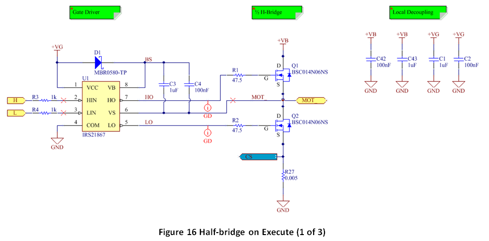
The IRS21867 was selected because of its robustness, especially for its tolerance to negative transient voltages. For the MOSFETs, the QFN 5x6 package (also known as 8-PowerTDFN and PG-TDSON-8) was selected for its small size, its wide industry acceptance and the convenience of doing bottom cooling.
The BSC014N06NS MOSFETs were selected for their availability, price, low RDSON and low gate capacitance. As a safety margin, MOSFETs rated for at least twice the bus voltage (28V Max) were selected. At 60V, the BSC014N06NS are protected in case of really bad inductive spikes.
The R1 and R2 gate resistors were selected from what could be called an “educated arbitrarily decision” as a compromise value between fast switching and slow switching. Switching too slowly can introduce shoot-through and increase switching losses, while switching too fast can increase the transient voltages generated (can lead to more noise, and to component destruction in extreme cases). The efficiency of the motor driver can be augmented by carefully selecting gate resistors and by doing a careful selection of semiconductors, but this optimization is outside of the scope of this work.
R27 is used for current sensing.
![]()
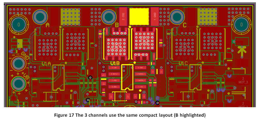
As can be seen on Figure 17 a large number of vias are used. They serve two purposes: thermal transfer and layer “tying”. This PCB has 6 layers:
- Layer 1: Top components, signals and small planes
- Layers 2 and 5: Ground planes
- Layer 3: Power. Top half is a +VB plane, Bottom half is a +5V plane.
- Layer 4: Mixed. In the context of the bridges, it is used for the MOT nets and for +VB.
- Layer 6: Bottom components, interface to the heat sink (so a maximum plane area is used around the bridges).
The critical power paths are always shared by a minimum of two layers.
[6] http://en.wikipedia.org/wiki/H_bridge
-
Trajectory generation: trapezoidal speed profile
09/07/2015 at 18:29 • 0 commentsPicture yourself in your car, going from one stop sign to the next. The fastest way to cover that distance would be to put the pedal to the ground, go as fast as possible and, at the last second, brake as hard as possible. Why isn’t that the prevailing way of driving? First, the accelerations would be way too high, you’d go from pulled in your seat to banging your head on the steering wheel. Second, unless you are driving a race car, the dynamics at play will prevent you from instantaneously reaching your top speed. You’ll need time to accelerate and decelerate.
A typical way to control robotic joints is to use a trapezoidal speed profile, which is quite similar to the profiles you’d get by driving your car: acceleration, constant speed, and deceleration.
![]()
In terms of math and logic the code is extremely simple. I wrote two Matlab scripts; the first one has all the math, and the second one loads experiments and calls the first one. To understand how I implemented this, read this code first, then dig in the C files.
Main function:
function [ spd, pos, acc ] = trapez_motion_2( pos_i, pos_f, spd_i, spd_max, a )
%Based on trapez_motion_1.m Now in a function
% Limitation(s): assumes 0 initial speed (spd_i is useless, should be 0)

    dt = 0.01;  %10ms
    skip_sspeed = 0;

    d_pos = pos_f - pos_i;          %Difference in position
    d_spd = spd_max - spd_i;        %Difference in speed
    a_t = d_spd / a;                %How long do we accelerate?
    a_t_discrete = a_t / dt        %   (in ticks)
    spd_inc = d_spd / a_t_discrete %Every tick, increase spd by
    %Position from acc:
    acc_pos = 0;
    for i = 1:a_t_discrete
        acc_pos = acc_pos + (i*spd_inc*dt);
    end
    acc_pos

    %It's possible to overshoot position if the acceleration is too low.
    %In that case we should sacrifice the top speed
    if((2*acc_pos) > d_pos)
        disp('Position overshoot')

        spd_max = sqrt(a*d_pos)

        %Redo the initial math:
        d_spd = spd_max - spd_i;        %Difference in speed
        a_t = d_spd / a;                %How long do we accelerate?
        a_t_discrete = a_t / dt        %   (in ticks)
        spd_inc = d_spd / a_t_discrete %Every tick, increase spd by
        %Position from acc:
        acc_pos = 0;
        for i = 1:a_t_discrete
            acc_pos = acc_pos + (i*spd_inc*dt);
        end
        acc_pos
    end

    cte_spd_pos = d_pos - 2*acc_pos;
    cte_spd_pos_discrete = (cte_spd_pos/spd_max) / dt
    if(cte_spd_pos_discrete < 0)
        disp('No steady speed!')
        skip_sspeed = 1;
    end

    %At this point all the parameters are computed, we can get the 3 plots
    vector_length = 2*length(a_t_discrete) + length(cte_spd_pos_discrete);
    spd = zeros(1,vector_length);
    spd(1) = spd_i;
    pos = zeros(1,vector_length);
    pos(1) = pos_i;
    acc = zeros(1,vector_length);
    acc(1) = a;
    %Acceleration:
    for i = 1:a_t_discrete
        tmp_spd = spd(end) + spd_inc;
        tmp_pos = sum(spd)*dt;
        tmp_acc = a;

        spd = [spd tmp_spd];
        pos = [pos tmp_pos];
        acc = [acc tmp_acc];
    end
    if(skip_sspeed == 0)
        %Constant speed
        for i = 1:cte_spd_pos_discrete
            tmp_spd = spd(end);
            tmp_pos = sum(spd)*dt;
            tmp_acc = 0;

            spd = [spd tmp_spd];
            pos = [pos tmp_pos];
            acc = [acc tmp_acc];
        end
    end
    %Negative Acceleration:
    for i = 1:a_t_discrete
        tmp_spd = spd(end) - spd_inc;
        tmp_pos = sum(spd)*dt;
        tmp_acc = -a;

        spd = [spd tmp_spd];
        pos = [pos tmp_pos];
        acc = [acc tmp_acc];
    end
end
And now the code the function that calls the previous script:
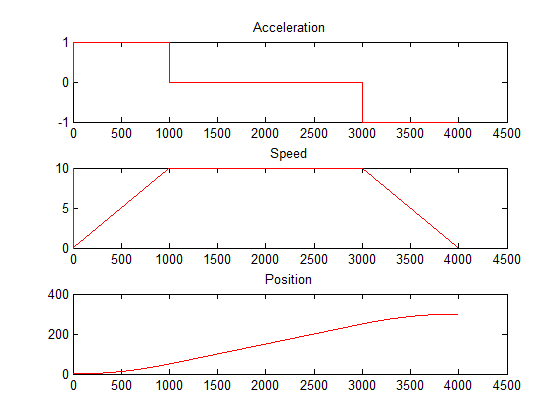
close all;
clear all;
clc;

% exp(1,:) = [1000,3000,0,700,150];
% exp(2,:) = [0,100,0,10,1];
% exp(3,:) = [0,500,0,10,1];
% exp(4,:) = [0,500,0,10,1];
exp(5,:) = [0,500,10,20,1];
% exp(6,:) = [0,300,0,15,5];
% exp(7,:) = [0,100,0,5,10];
% exp(8,:) = [0,5,0,5,1];
dim = size(exp);
max_i = dim(1);

for i = 1:max_i

    str = sprintf('Experiment #%i',i);
    disp(str)
    [spd1 pos1 acc1] = trapez_motion_2(exp(i,1),exp(i,2),exp(i,3),exp(i,4),exp(i,5));

    figure()
    subplot(3,1,1)
    plot(acc1, 'r')
    title('Acceleration')
    subplot(3,1,2)
    plot(spd1, 'r')
    title('Speed')
    subplot(3,1,3)
    plot(pos1, 'r')
    title('Position')

end
The beauty of Matlab is that it’s so powerful and simple. You can quickly prove your algorithm… but will it work in real life? In that case, my first C implementation had issues with integer rounding that created a lot of problems.
![]()
Those sharp transitions created a lot of vibration and instability on the prosthetic knee I was using as a test bench!
Here's the full C implementation, starting with trapez.h and followed by trapez.c:
//****************************************************************************
// MIT Media Lab - Biomechatronics
// Jean-Francois (Jeff) Duval
// jfduval@mit.edu
// 05/2015
//****************************************************************************
// trapez: trapezoidal trajectory generation
//****************************************************************************

#ifndef TRAPEZ_H_
#define TRAPEZ_H_

//****************************************************************************
// Include(s):
//****************************************************************************

//****************************************************************************
// Public Function Prototype(s):
//****************************************************************************

long long trapez_gen_motion_1(long long pos_i, long long pos_f, long long spd_max, long long a);
long long trapez_get_pos(long long max_steps);

//****************************************************************************
// Definition(s):
//****************************************************************************

#define TRAPEZ_DT           	0.001		//Trapezoidal timebase. Has to match hardware!
#define TRAPEZ_ONE_OVER_DT  	1000
#define SPD_FACTOR          	10000		//Scaling for integer
#define ACC_FACTOR          	10000

#endif // TRAPEZ_H_
//**************************************************************************** // MIT Media Lab - Biomechatronics // Jean-Francois (Jeff) Duval // jfduval@mit.edu // 05/2015 //**************************************************************************** // trapez: trapezoidal trajectory generation //**************************************************************************** //Work based on trapez_gen_x.m, translated in C //JFDuval 06/17/2014 //**************************************************************************** // Include(s) //**************************************************************************** //Comment the next line to use in your application: //#define DEBUGGING_OUTPUT #include <stdio.h> #include <stdint.h> #include <stdlib.h> #include <math.h> #include "trapez.h" //#include "main.h" //**************************************************************************** // Local variable(s) //**************************************************************************** //Common variables - careful, do not change "manually"! long long d_pos = 0, d_spd = 0, a_t = 0, a_t_discrete = 0, spd_inc = 0, acc_pos = 0, acc = 0; long long init_pos = 0, cte_spd_pos = 0, cte_spd_pos_discrete = 0; long long skip_sspeed = 0; long long pos_step = 0; long long trapez_transitions[3] = {0,0,0}; long long sign = 0; //**************************************************************************** // Private Function Prototype(s): //**************************************************************************** static long long trapez_compute_params(long long pos_i, long long pos_f, long long spd_max, long long a); //**************************************************************************** // Public Function(s) //**************************************************************************** //Based on trapez_motion_2.m //Assumes 0 initial speed long long trapez_gen_motion_1(long long pos_i, long long pos_f, long long spd_max, long long a) { long long abs_d_pos = 0, abs_acc_pos = 0, dual_abs_acc_pos = 0; //spd_max & a have to be positive spd_max = llabs(spd_max); a = llabs(a); //Compute parameters (in global variables) trapez_compute_params(pos_i, pos_f, spd_max, a); //Absolute values abs_d_pos = llabs(d_pos); abs_acc_pos = llabs(acc_pos); dual_abs_acc_pos = 2*abs_acc_pos; #ifdef DEBUGGING_OUTPUT printf("d_pos = %lld, abs_d_pos = %lld.\n", d_pos, abs_d_pos); printf("1) acc_pos = %lld, abs_acc_pos = %lld.\n", acc_pos, abs_acc_pos); #endif //It's possible to overshoot position if the acceleration is too low. //In that case we should sacrifice the top speed if(dual_abs_acc_pos > abs_d_pos) { #ifdef DEBUGGING_OUTPUT printf("Position overshoot.\n"); #endif //New top speed: spd_max = sqrt(a*abs_d_pos); #ifdef DEBUGGING_OUTPUT printf("New spd_max: %lld.\n", spd_max); #endif //Redo the initial math: //Compute parameters (in global variables) trapez_compute_params(pos_i, pos_f, spd_max, a); //Absolute values (they probably changed) abs_d_pos = abs(d_pos); abs_acc_pos = abs(acc_pos); dual_abs_acc_pos = 2*abs_acc_pos; } //Plateau - constant speed #ifdef DEBUGGING_OUTPUT printf("d_pos = %lld, abs_d_pos = %lld.\n", d_pos, abs_d_pos); printf("2) acc_pos = %lld, abs_acc_pos = %lld.\n", acc_pos, abs_acc_pos); #endif cte_spd_pos = abs_d_pos - (2*abs_acc_pos); cte_spd_pos_discrete = (SPD_FACTOR*cte_spd_pos/spd_max)*TRAPEZ_ONE_OVER_DT; cte_spd_pos_discrete = cte_spd_pos_discrete / SPD_FACTOR; #ifdef DEBUGGING_OUTPUT printf("cte_spd_pos = %lld, cte_spd_pos_discrete = %lld.\n", cte_spd_pos, cte_spd_pos_discrete); #endif if(cte_spd_pos_discrete < 0) { cte_spd_pos_discrete = 0; #ifdef DEBUGGING_OUTPUT printf("No steady speed!\n"); #endif } //Transitions: trapez_transitions[0] = a_t_discrete; trapez_transitions[1] = a_t_discrete + cte_spd_pos_discrete; trapez_transitions[2] = 2*a_t_discrete + cte_spd_pos_discrete; #ifdef DEBUGGING_OUTPUT printf("tr[0] = %lld, tr[1] = %lld, tr[2] = %lld.\n", trapez_transitions[0], trapez_transitions[1], trapez_transitions[2]); #endif pos_step = 0; //Variable used to output the current position command return (2*a_t_discrete + cte_spd_pos_discrete); //Returns the number of steps } //Runtime function - gives the next position setpoint long long trapez_get_pos(long long max_steps) { static long long tmp_spd = 0, last_tmp_spd = 0, tmp_pos = 0; long long position = 0; static long long pos_integral = 0; //At this point all the parameters are computed, we can get the 3 plots //First time: if(pos_step == 0) { tmp_spd = 0; last_tmp_spd = 0; tmp_pos = 0; pos_integral = 0; #ifdef DEBUGGING_OUTPUT printf("pos_step = 0, pos_integral = %lld.\n", pos_integral); #endif } //Acceleration: if(pos_step <= trapez_transitions[0]) { last_tmp_spd = tmp_spd; tmp_spd = last_tmp_spd + spd_inc; } //if(skip_sspeed == 0) //ToDo useful? { //Constant speed //last_tmp_spd = tmp_spd; if((pos_step >= trapez_transitions[0]) && (pos_step <= trapez_transitions[1])) { tmp_spd = last_tmp_spd; } } //Negative Acceleration: if((pos_step >= trapez_transitions[1]) && (pos_step <= trapez_transitions[2])) { last_tmp_spd = tmp_spd; tmp_spd = last_tmp_spd - spd_inc; } if(pos_step <= max_steps) { //Ready for next one. pos_step++; //Common math: pos_integral += tmp_spd; tmp_pos = pos_integral/(TRAPEZ_ONE_OVER_DT * SPD_FACTOR); position = tmp_pos + init_pos; #ifdef DEBUGGING_OUTPUT if(pos_step < 10) printf("pos_step = %lld, pos_integral = %lld, position = %lld.\n", pos_step, pos_integral, position); #endif } else { position = tmp_pos + init_pos; } //New setpoint return position; } //**************************************************************************** // Private Function(s) //**************************************************************************** //Computes all the parameters for a new trapezoidal motion trajectory //Called by trapez_gen_motion_1() static long long trapez_compute_params(long long pos_i, long long pos_f, long long spd_max, long long a) { long long tmp = 0, i = 0; //Sign if(pos_f < pos_i) sign = -1; else sign = 1; acc = a; init_pos = pos_i; d_pos = pos_f - pos_i; //Difference in position d_spd = spd_max ; //Difference in speed a_t = (ACC_FACTOR*d_spd) / a; //How long do we accelerate? a_t_discrete = a_t * TRAPEZ_ONE_OVER_DT / ACC_FACTOR; // (in ticks) //a_t_discrete = a_t; //Simplification of *100/100 spd_inc = (sign*SPD_FACTOR*d_spd) / a_t_discrete; //Every tick, increase spd by #ifdef DEBUGGING_OUTPUT printf("d_spd = %lld, a_t_discrete = %lld, spd_inc = %lld, d_pos = %lld.\n", d_spd, a_t_discrete, spd_inc, d_pos); #endif acc_pos = 0; for(i = 0; i < a_t_discrete; i++) { tmp += spd_inc; //tmp = i*spd_inc; acc_pos = acc_pos + tmp; } acc_pos = acc_pos / (SPD_FACTOR * TRAPEZ_ONE_OVER_DT); //Combine terms #ifdef DEBUGGING_OUTPUT printf("acc_pos = %lld (2x = %lld), %f%% of d_pos.\n", acc_pos, (2*acc_pos), (float)(2*acc_pos*100/d_pos)); #endif return 0; }As you can see, I’m multiplying everything by a big factor to use integer math (way more efficient than floating point math) and I scale it back down once I’m done computing.At runtime, in my time shared while() loop (see Managing timing: how to sequence tasks for more details) I can get a new setpoint and use it for my controllers. The trajectory is only calculated when I initiate a new motion (usually after receiving a command from FlexSEA-Manage or -Plan).
				//Case 5: Quadrature encoder & Position setpoint
				case 5:

					#ifdef USE_QEI1

					//Refresh encoder readings
					encoder_read();

					#endif	//USE_QEI1

					#ifdef USE_TRAPEZ

					if((ctrl.active_ctrl == CTRL_POSITION) || (ctrl.active_                                        ctrl == CTRL_IMPEDANCE))
					{
						//Trapezoidal trajectories (can be used for bot                                                h Position & Impedance)
						ctrl.position.setp = trapez_get_pos(steps);	                                        //New setpoint
					}

					#endif	//USE_TRAPEZ

					break;

				//Case 6: P & Z controllers, 0 PWM
				case 6:

					#ifdef USE_TRAPEZ

					if(ctrl.active_ctrl == CTRL_POSITION)
					{
						motor_position_pid(ctrl.position.setp, ctrl.pos                                                ition.pos);
					}
					else if(ctrl.active_ctrl == CTRL_IMPEDANCE)
					{
						//Impedance controller
						motor_impedance_encoder(ctrl.impedance.setpoint                                                _val, ctrl.impedance.actual_val);
					}

					#endif	//USE_TRAPEZ

					//If no controller is used the PWM should be 0:
					if(ctrl.active_ctrl == CTRL_NONE)
					{
						motor_open_speed_1(0);
					}

					break;
And that’s it! You now have a complete example of a trajectory generator, both in Matlab and C, that works in the real life.
Now, please note that a better strategy is to use s-curve trajectories to minimize the jerk. I didn’t implement that yet, but feel free to contribute to FlexSEA by coding it! Some reference here: On Algorithms for Planning S-curve Motion Profiles.
-
FlexSEA-Plan
09/07/2015 at 16:44 • 0 commentsFlexSEA-Plan is an embedded computer used for high-level computing. It boasts a powerful processor and can run an operating system such as Linux. Developing code on this platform is similar to the regular (i.e. non-embedded) software development process. High-level languages such as Python can be used, saving experimental data is as simple as writing to a text file and interacting with the system can be done via USB or WiFi. FlexSEA-Plan should be used when ease of development is important, and when complex algorithms and control schemes require significant computing power.
The initial plan was to design a custom embedded computer with only the features required for our application. To start experimenting before designing, the BeagleBone Black was selected. It is economical ($55), widely available, open-source hardware (with full documentation available) and its processor, the TI AM3358, has two Programmable Realtime Units (PRU) that can be used to efficiently communicate with peripherals, making it a perfect reference for a custom design. By removing multimedia features and optimizing connectors its size (89 x 55 x 15.4mm) can be greatly reduced.
While the design efforts were focused on FlexSEA-Manage and FlexSEA-Execute, the Internet of Things (IoT) wave grew stronger. Smaller embedded computers were released, with price tags low enough to be embedded in typical appliances. One example is the Intel Edison. At 35 x 25 x 4mm it has a 500MHz processor, 1GB of RAM, 4GB of FLASH, Bluetooth and WiFi. It was decided not to design a custom embedded computer but to rather use a standard communication interface (SPI) that would allow the user to select any product on the market. Processing power can easily be added to the FlexSEA system as new embedded computers become available.
-
Working toward FlexSEA-Execute 0.2
09/06/2015 at 21:34 • 0 commentsIn The evolution of FlexSEA prototypes I’m showing the first 3 generations of FlexSEA-Execute designs. While the 3rd generation, FlexSEA-Execute 0.1 (I know, it’s the third one but I named it 0.1 because I changed the naming convention and it felt wrong to start with 0.3!) is stable and functional, nothing is ever perfect. In my thesis I wrote down:
List of modifications that do not require circuit modifications (only BOM changes):
- Lower the I²C resistor pull-ups (R45, R46) to 1.8kΩ (currently 4.7kΩ)
- Change the IO protection resistors (R10-R13, R64, R65) to 120Ω (currently 100Ω)
- Less resistive PTCs (F1, F2)
- Lower the Gate resistor values by at least half. More calculations and testing is required to find the optimal value.
List of modifications requiring circuit modifications:
- The 400kHz I²C limit on the MPU-6500 is slowing down the bus. If a new IMU has to be selected a 1MHz version should be considered.
- RGB LED: poor color balance. The next design should use 243/249/412Ω.
- Add a second green LED to unify the user interface with Manage.
- Add an external filtering capacitor for the Delta Sigma converter (0.1 to 1.0µF, see component datasheet).
- Add SWD (P1[3]) to the PSoC 5 SWD connector (J9). The Serial Viewer isn’t supported yet but will be convenient in the future.
- The ‘+5V’ supply should be measured.
- The RS-485 transceivers (U4, U10, U11) should use the 8-SON package to save board space and unify the BOM with Manage.
- The position of the SWD connectors (J5, J9) is not convenient. They should be on the top side. Swapping their position with the RS-485 transceivers would be convenient.
- Many expansion pins are on port 12. They are SIO and not GPIO (no analog features). Most of the expansion signals should support analog inputs.
Of course, since then I had many improvement ideas. But first, I need to run a series of experiment to confirm/infirm some parts of the design:
- Test the triple channel RS-485
- Test RGB resistor values
- Gate resistor values
- Reliability test with the lower gate resistors
- Thermal/load test with the lower gate resistors
- How should I interface a wireless module?
- Test the shorted lead protection
- Single stage SG amplifier?
- Test with external SPI circuits
- How can I use a Manage board with minimal wires? Or directly connect Plan?
- Evaluate LM510x chips to get smaller drivers
- Is there a better PSoC 5 available?
- PSoC 4 with Bluetooth to replace the co-processor???
- Shorted leads: better MOSFETs?
- How can I support higher voltages? Currently limited by the LM25011 (42V). 48V would be great.
- Can I add memory to log experiments?
Other than minor technical fixes, the biggest improvements will be the wireless communication and the high supply voltage. Once I’m done with that list (spoiler alert, I already found answers for some of the questions!) I’ll implement all the changes in Altium and roll-out a new batch of Execute boards. This should keep me busy for the next few weeks!
Do you see something missing? What feature would you integrate?
-
The evolution of FlexSEA prototypes
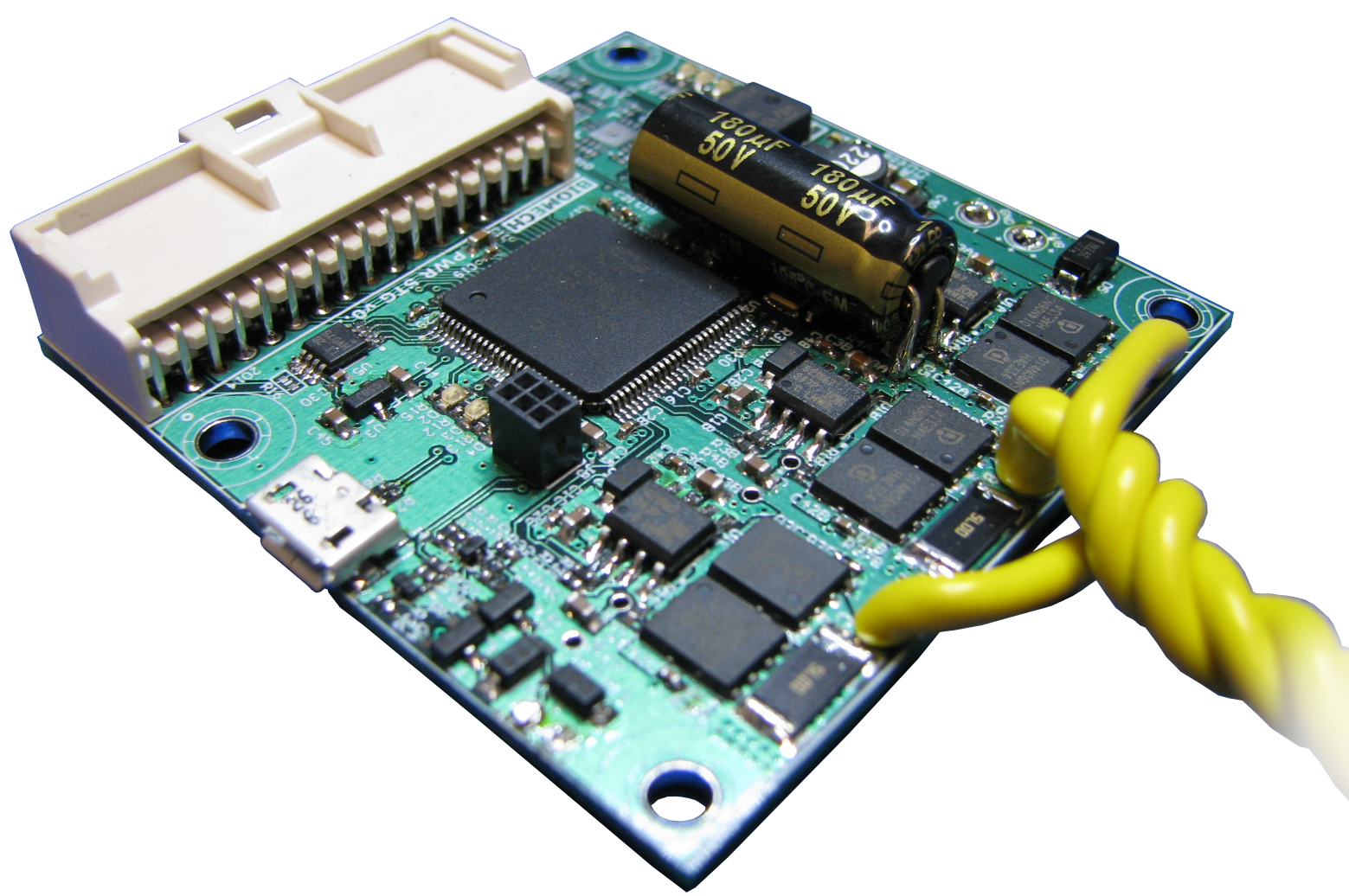
09/06/2015 at 18:42 • 0 commentsBefore I adopted the business naming convention (Plan, Manage & Execute) the motor drivers were named PWR_STG, short for Power Stage. The FlexSEA-Execute 0.1 boards that you can see in most of the pictures is the 3rd prototype generation. How did I start from scratch and end up there?
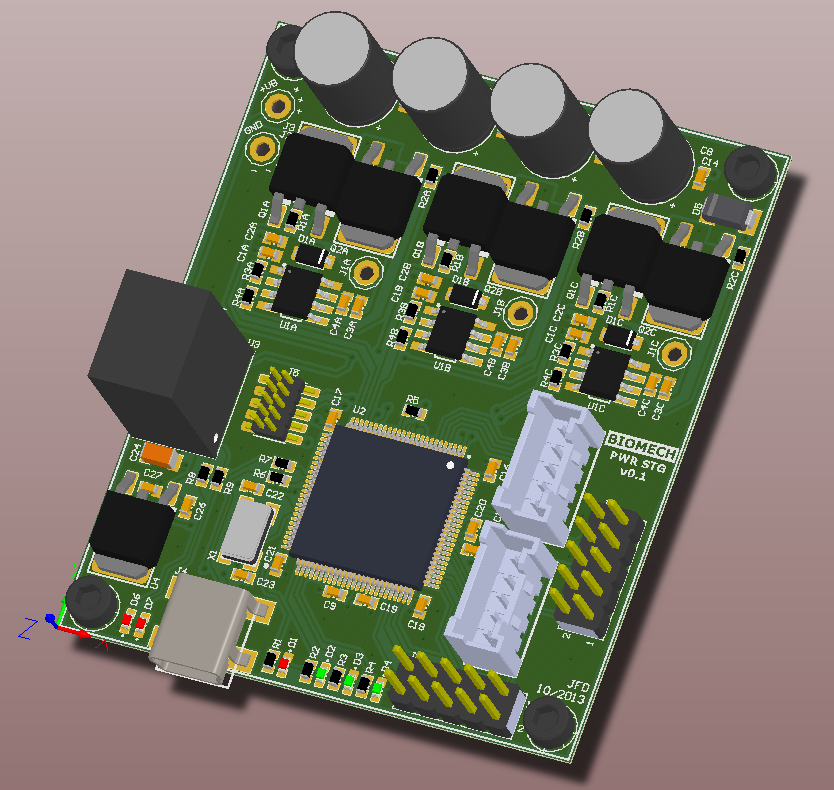
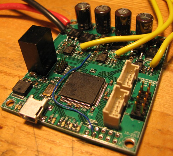
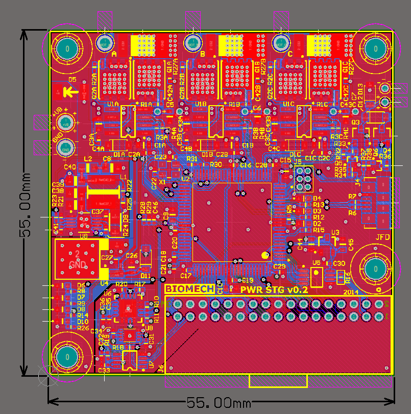
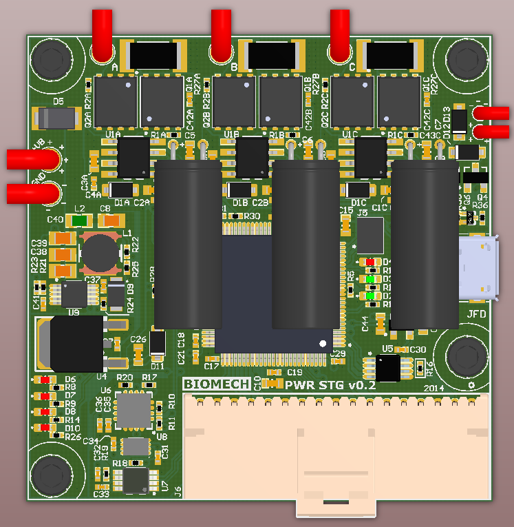
10/2013: PWR_STG_0_1
Goal(s): to get started! I needed to force myself to work harder, and I needed a platform to test my software.
Strategy/details: testing the schematic and my libraries was important. I kept the layout as simple as possible (2 layers, low density) to facilitate hand assembly. Passive components were 0603. The big black box on the left is a V7810, a DC/DC regulator intended to replace the venerable 7810. For the 10V to 5V conversion I was using a linear regulator, LM7805 (that’s the big DPAK package on the left). Connectors were big and un-optimized (motor wires are in the middle of the board). I knew that I couldn’t draw much current from this board, but that was not the point.
PCB layout - 2D PCB layout - 3D Prototype ![]()
![]()
![]()
You can read more about this design on my How To Make (almost) Anything pages (I saved time by using my research for weekly assignments). During Week 6: Electronics Design I talk about PSoC selection and design choices, on Week 8: Embedded Programming I have a brief progress report and on Week 11: Output Devices I show a nice demo: “writing” text with a brushless DC motor (including intro to BLDC motors, PID basics, Matlab character generation, 2D plotting, etc).
02/2014: PWR_STG_0_2
Goal(s): add sensor signal processing, communication interface (RS-485), better power supplies and do a more compact layout. This revision had to be close to the end product.
Strategy/details: I did test PCBs for some of the modules (strain gauge amplifier, DC/DC power supply, RS-485 interface) and, after testing, integrated these design modules in the PWR_STG_0_2 project. I picked better components and spent more time on the layout (more compact, better thermal engineering). I kept things simple as I knew I would hand-assemble the first prototypes.
PCB layout - 2D PCB layout - 3D Prototype ![]()
![]()
![]()
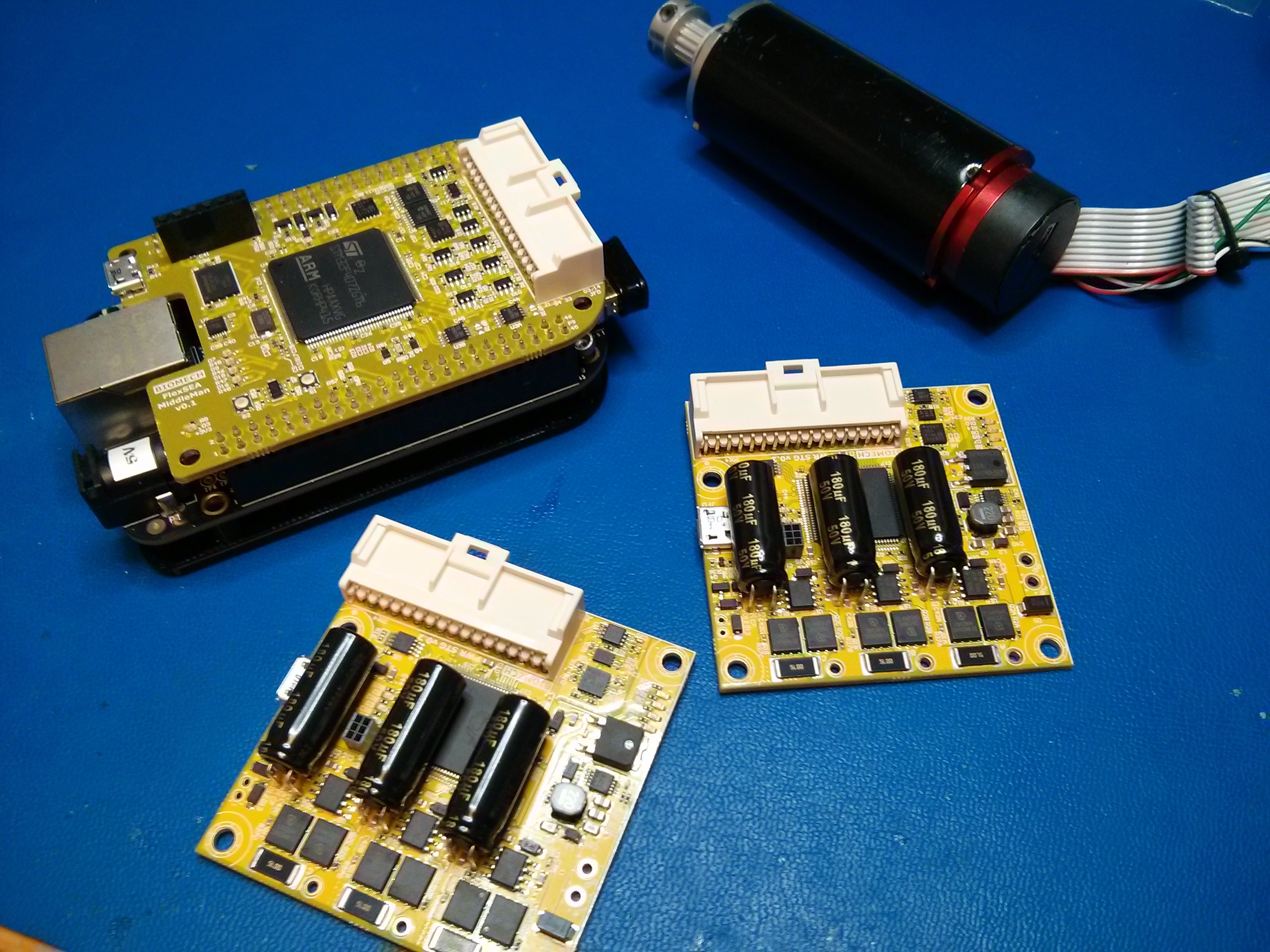
I was really happy when I started using the boards in prosthesis, without any hardware patches! I had Nexlogic build a batch of 10 kits (Middleman, later named Manage, and Execute boards) with a nice yellow soldermask:
A lot of the FlexSEA software was developed on these boards. Then I needed more…![]()
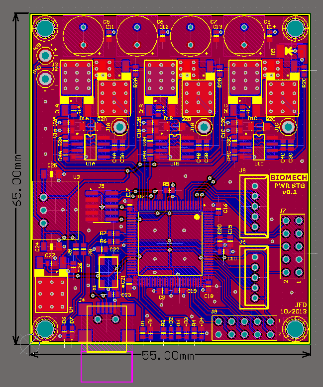
11/2014: FlexSEA-Execute 0.1
Goal(s): add safety features, optimize connectors, smaller product, easy to manufacture.
Strategy/details: in this revision I introduced the PSoC 4 safety co-processor, replaced a linear regulator by a DC/DC, fixed the strain gauge amplifier, added shorted-lead protections, selected denser connectors, designed a mounting plate/heatsink, added internal sensing, an IMU, etc… lots of modifications! The PCB is now 6 layers and I have a lot of 0402 and QFN parts, hand-assembly wouldn’t have been reliable (the power plane make it hard) so I outsourced everything to Nexlogic.
PCB layout - 2D PCB layout - 3D Prototype ![]()
![]()
![]()
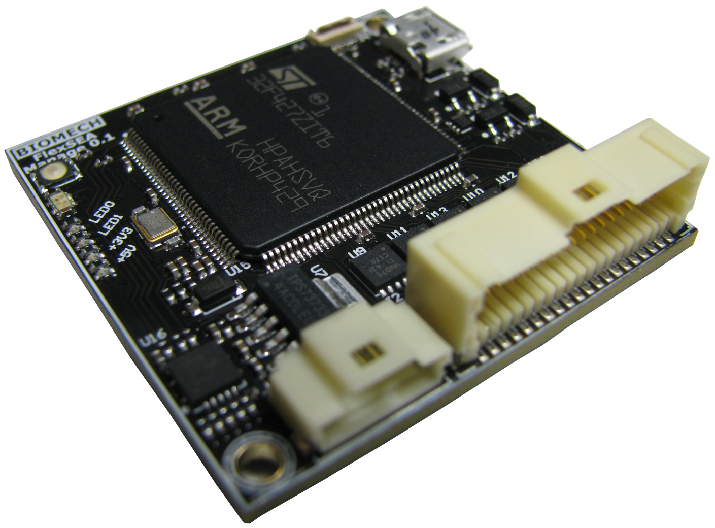
They also produced the Manage 0.1 board (now much much smaller than the Beagle Bone shield that you saw previously!):
And that's it! I'm now working on FlexSEA-Execute 0.2, expect a new project log soon...![]()
-
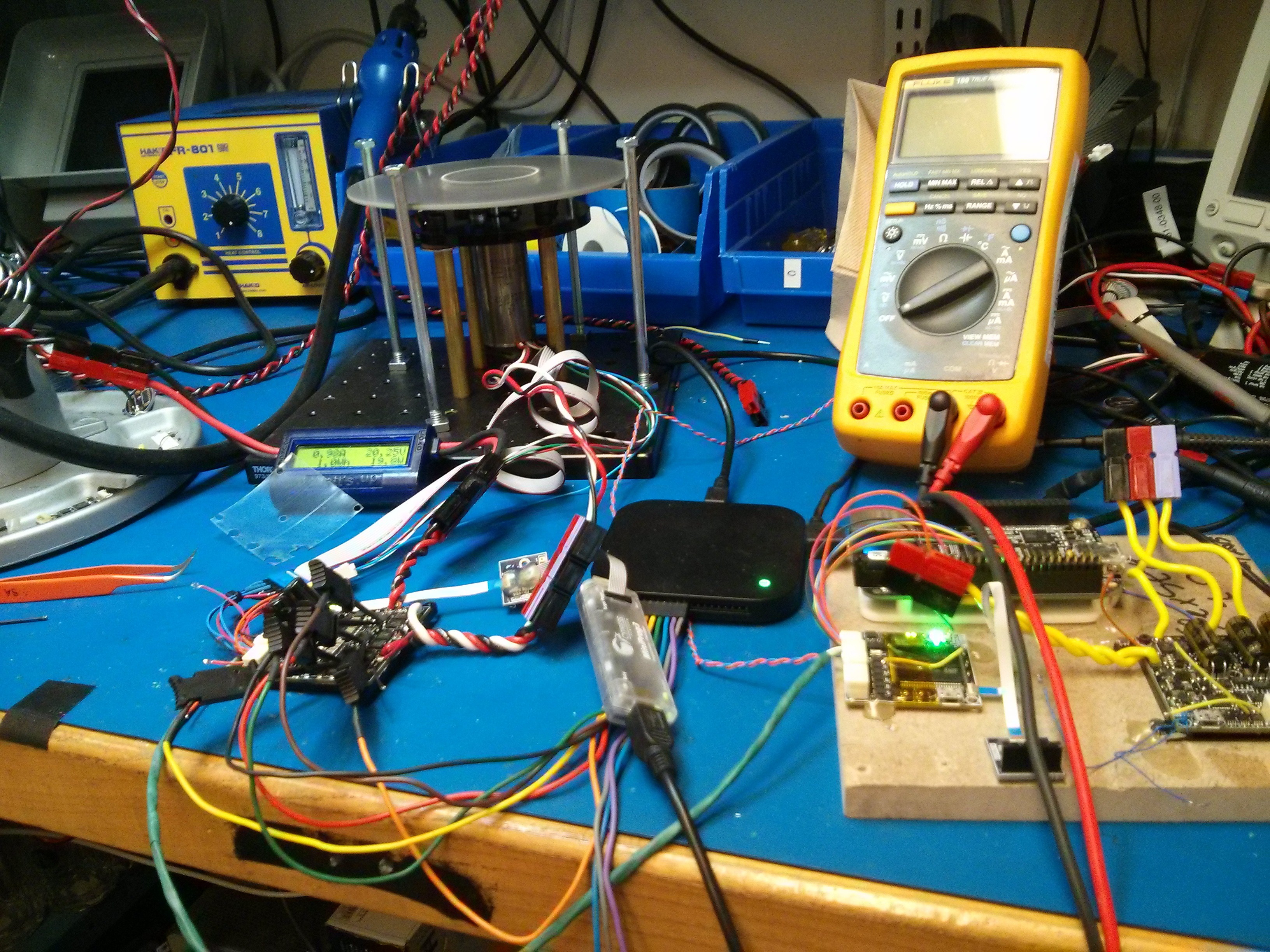
It’s Friday! Time for some messy prototyping/testing pictures.
09/04/2015 at 19:18 • 0 commentsWhat you see in my thesis and in my project logs is the final result. To keep it real, I decided to share with you some “action shots” taken during testing and prototyping of the different FlexSEA boards.
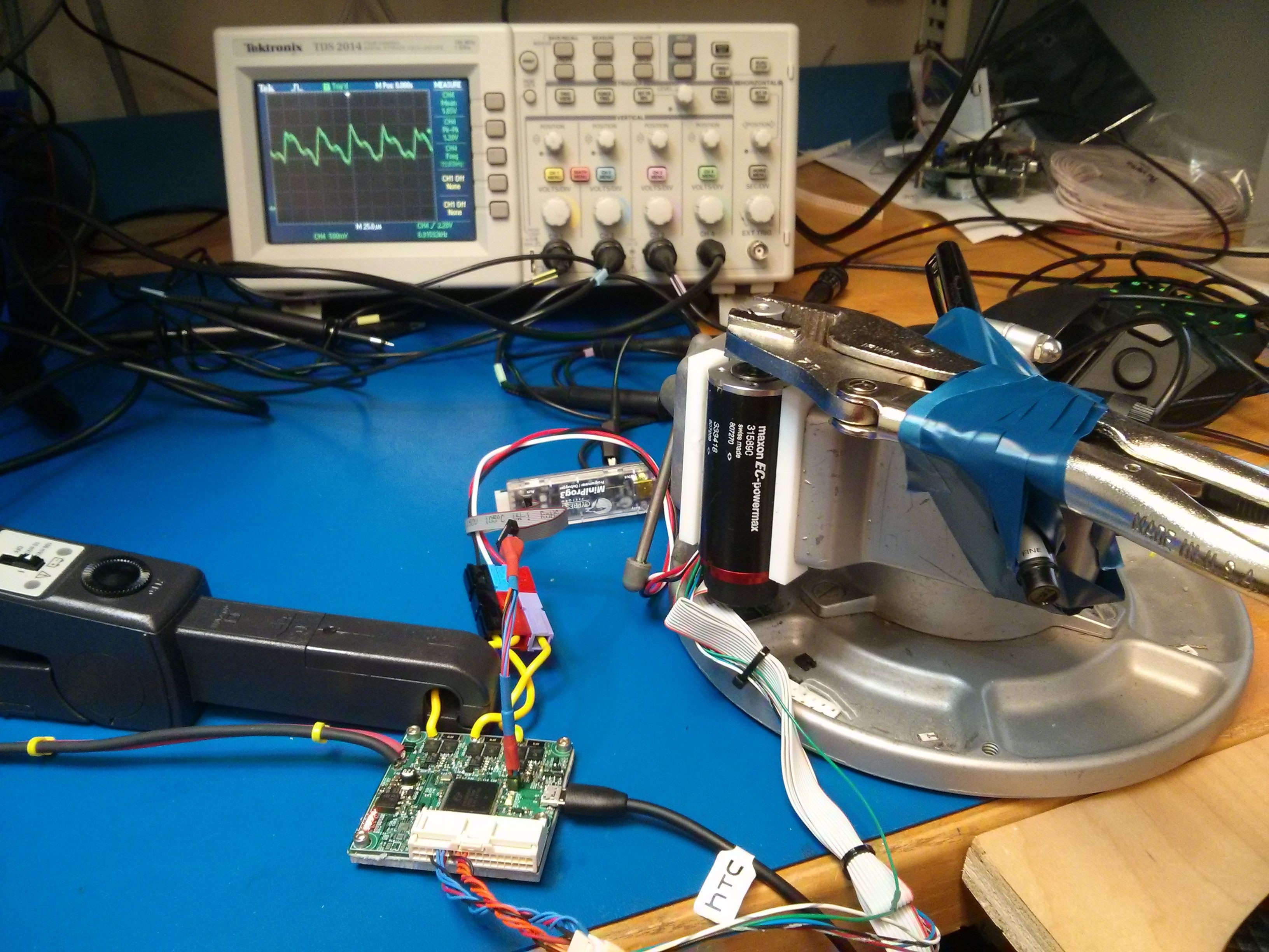
![]()
This one doesn’t look too bad… until you realized that I’m holding the motor shaft fixed with vise-grips, a pen and electrical tape. A few weeks after that I designed the test bench that you can see in Current Controller: Software.
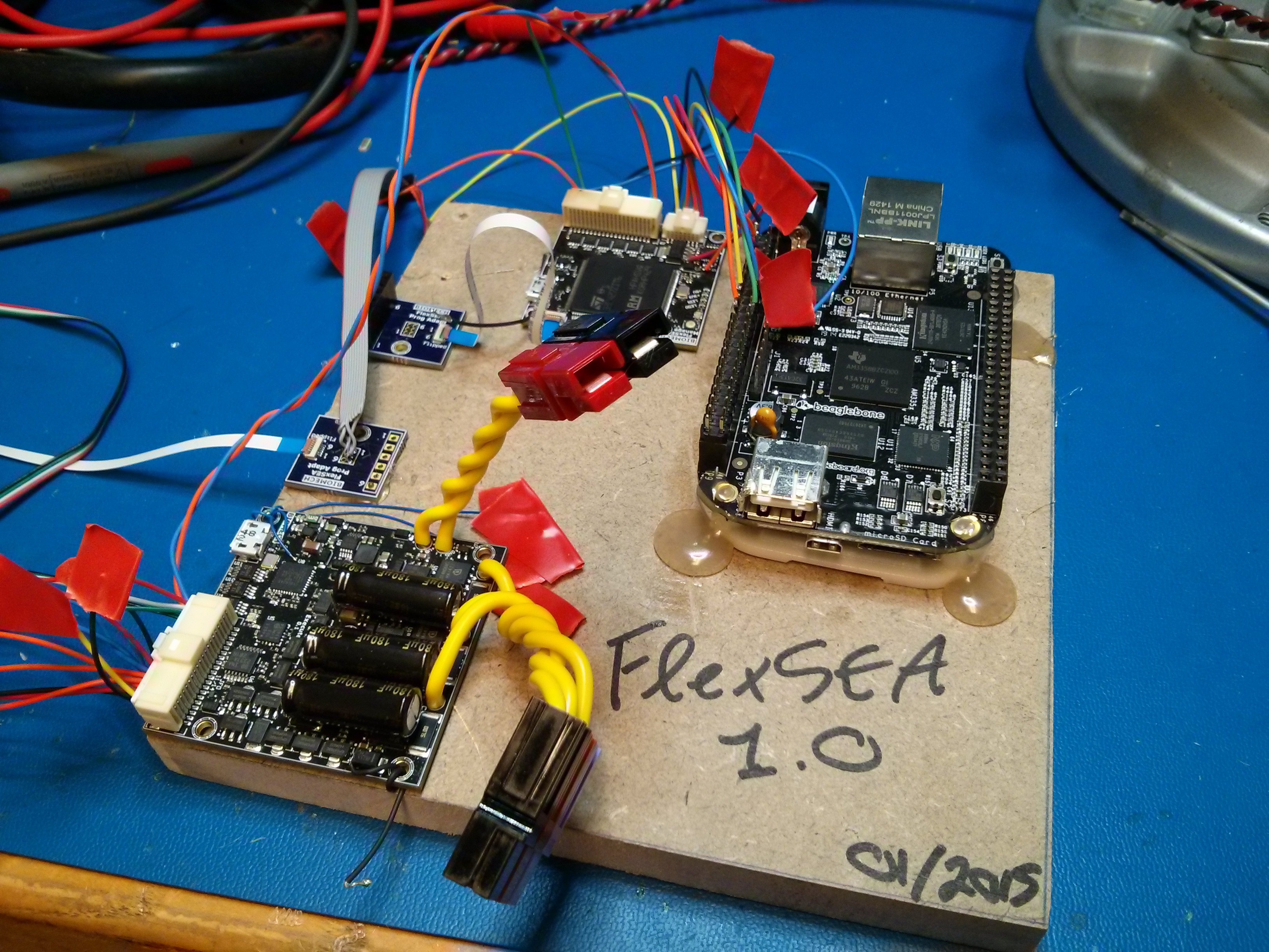
To test the circuits I usually hot-glue them to scrap pieces of MDF. No time for screws! Ugly, but functional.
![]()
![]()
Here you can see a FlexSEA-Execute board covered with test probes, a RC-Hobby Wattmeter and a big flywheel used to characterize the BLDC motor at high currents. The tall bolts act as a cage in case the flywheel… well, starts flying.
![]()
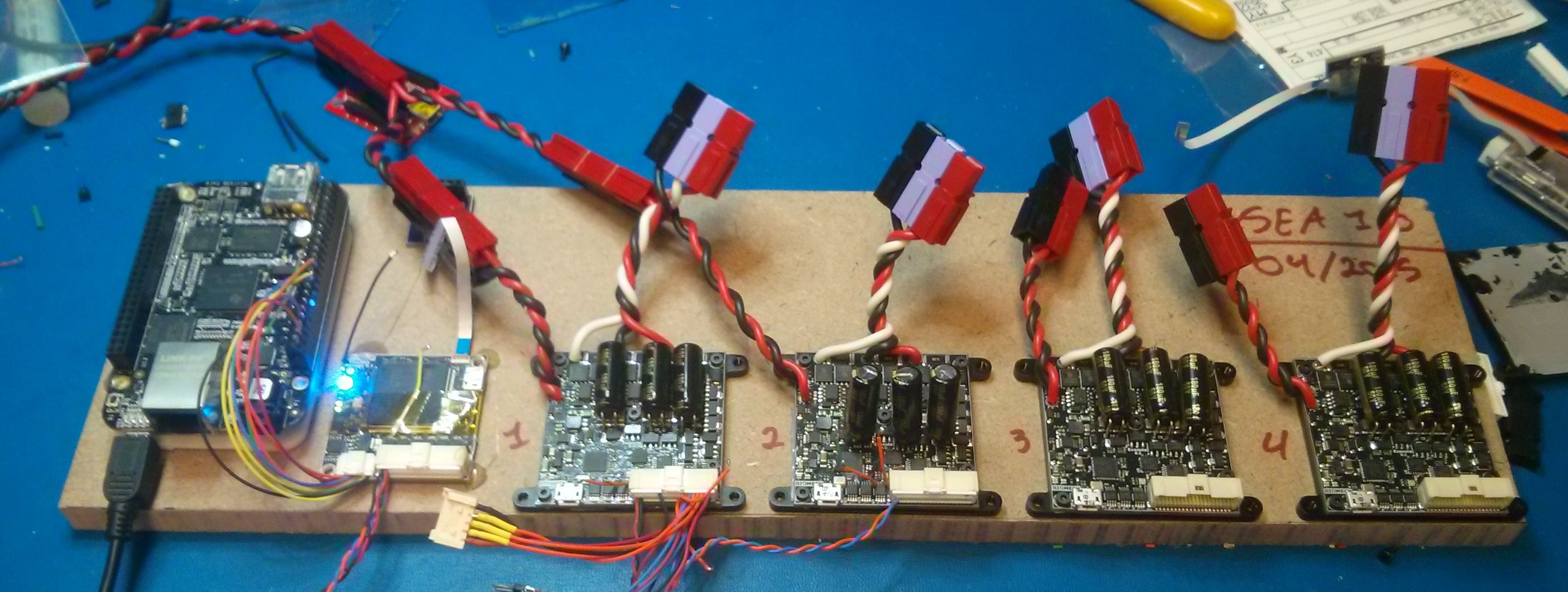
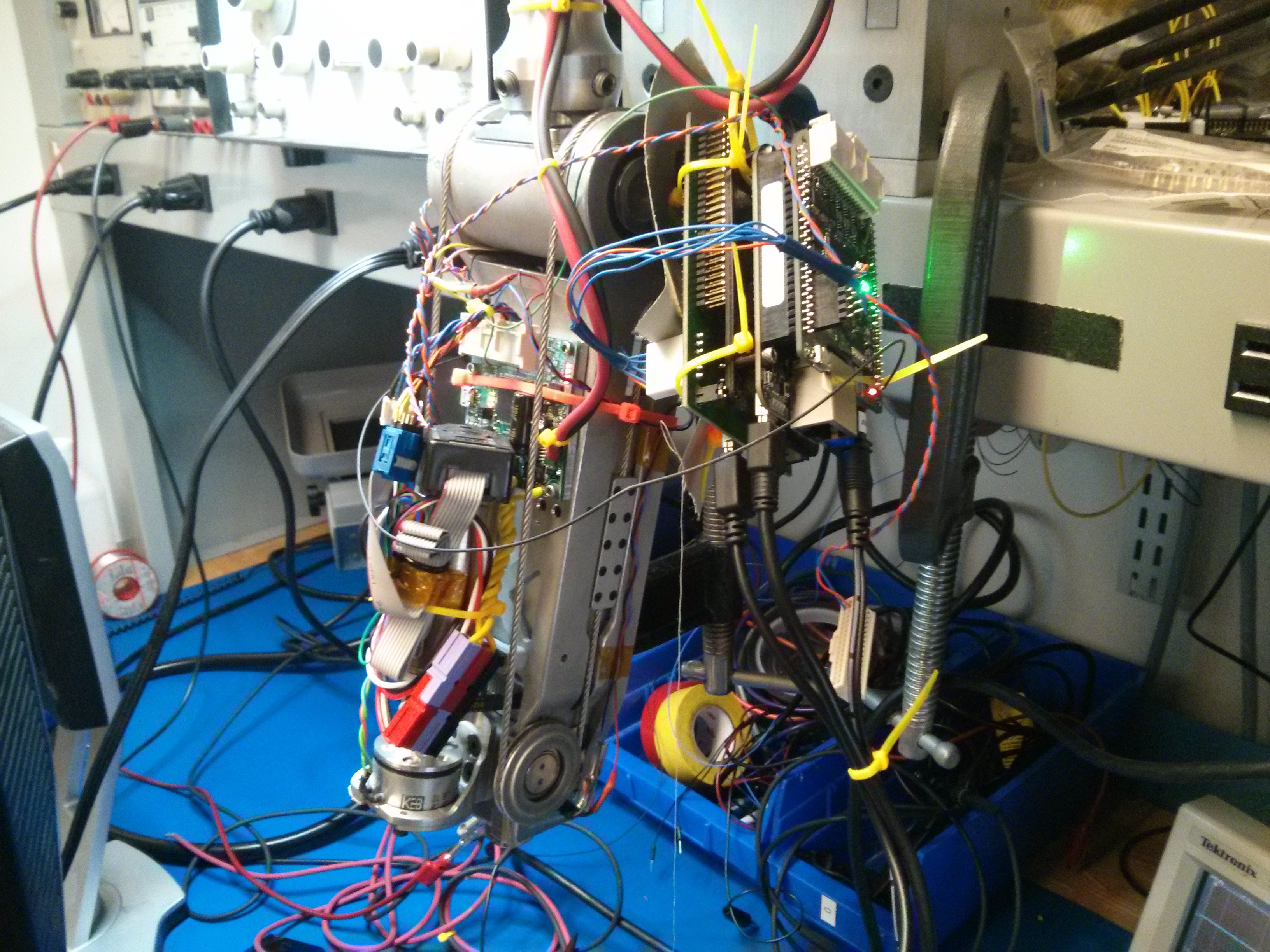
And finally, sometimes there is no time for wire management or mechanical integration!
![]()
![]()
Have a great weekend!
-
MOSFET Power Dissipation and Temperature
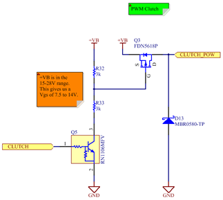
09/04/2015 at 19:03 • 0 commentsIn certain designs we want to use a clutch to hold joints still with a minimal amount of power. The power required to engage an electro-magnetic clutch is higher than the power required to keep it locked. We are using a MOSFET switch with PWM to control the average voltage applied to the clutch. What power rating do we need for this MOSFET?
Side note: why use a high-side P-MOSFET? The use of a high-side switch is preferred because it is typical to link the metal chassis of prostheses to ground and some clutches have their casing grounded. Using a high-side switch can simplify the electromechanical integration. The power requirements being low, it is possible to use a P-Channel MOSFET as a switch (N-MOSFET have better specs and are always used for high power applications, such as the motor bridge). D13 is used as a free-wheeling diode for inductive loads, as a protection for Q3.
![]()
P-MOSFET power dissipation:
The clutched used in the experimental setup is rated for 24V 250mA 6W. The unit in hand was tested at 242mA. To accommodate bigger clutches (and other output devices) the calculations will be done for 24V 10W (417mA), used at 10V. The current at 10V will be 174mA.
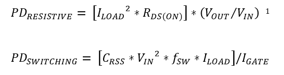
Using an FDN5618P P-MOSFET:
![]()
Where:
ILOAD: 174mA
VOUT/VIN = D = 10V/24V = 0.42
RDS(ON) = 0.315 Ω (worst case)
CRSS: 19pF
VIN: 24V
fSW: 20kHz
Igate: 10.9mA
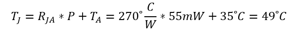
We obtain & . The total power dissipation is 7.5mW. If the clutch is powered at 24V 10W (no switching) the dissipation will be 55mW. The thermal resistance of the SuperSOT-3 package, from junction to ambient, is 270°C/W.
![]()
49C is way below the maximum junction temperature, we do not need to worry about thermal constraints and we can use the FDN5618P P-MOSFET for this application. I used a clutch as an example, but keep in mind that the math is the same for other output devices.
Note: Formulas based on http://electronicdesign.com/boards/calculate-dissipation-mosfets-high-power-supplies
FlexSEA: Wearable robotics toolkit
OSHW+OSS to enable the next generation of powered prosthetic limbs and exoskeletons. Let’s make humans faster/better/stronger!


 DC motors are commonly driven by a circuit called an H-Bridge. An H bridge is an electronic circuit that enables a voltage to be applied across a load in either direction. Closing S1 and S4 will make the motor turn in one direction, while closing S2 and S3 will make it rotate in the opposite direction. Closing S1 and S3, or S2 and S4, can be used to brake the motor. Closing S1 and S2, or S3 and S4, will create a short circuit on the power supply and can lead to catastrophic failure.