Open Source FFT Spectrum Analyzer

An error regarding the g_scale for calculating g from accelerometer voltage was pointed and corrected by Steve Ferry (thank you Steve).

adc_resolution = 3.3 / 1024 # Vref = 3.3V, 10 bit ADC.

accelerometer_sensitivity = 1000/300 # 300 mv/g

g_scale = adc_resolution * accelerometer_sensitivity = (3.3 / 1024) * (1000/300)

The Python 3 program has been corrected with this new value.

I think the mistake was to assume that +-3g would cover the whole ADC range, but it will cover only around 2 V, not all the 3.3 V (Vref) range.

Looking through the ADXL335 datasheet, the output is ratiometric (proportional to supply voltage), and the 300 mV/g is the approximate value using a 3.0 V supply. This numbers can have around 10% variation between devices, so I think that an additional correction factor will have to be introduced and calculated (calibrated) for each different accelerometer used.

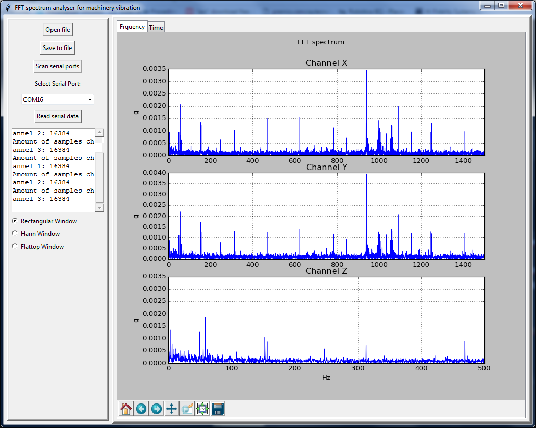
I have added a third axis to the spectrum analyzer. The atMega328 (Arduino Nano) program is adxl335_3can_01_en.c. The Python 2.7 program is fft_spectrum_gui_3can.py.

I also made a version of the three axis analyzer that works with Python 3.5, fft_spectrum_gui_3can_py3_01.py.

There is also a file with sampled data for testing purposes datos_3can_20-12-2016__11_39_50.txt. Works with both versions of the 3 axis FFT analyzer.

Notice that the accelerometer Z axis is limited to 500 Hz.

This files are also available on GitHub at https://github.com/ariquezada/FFT-spectrum-analyzer/tree/master/3_axis.

The screen shot is shown below.

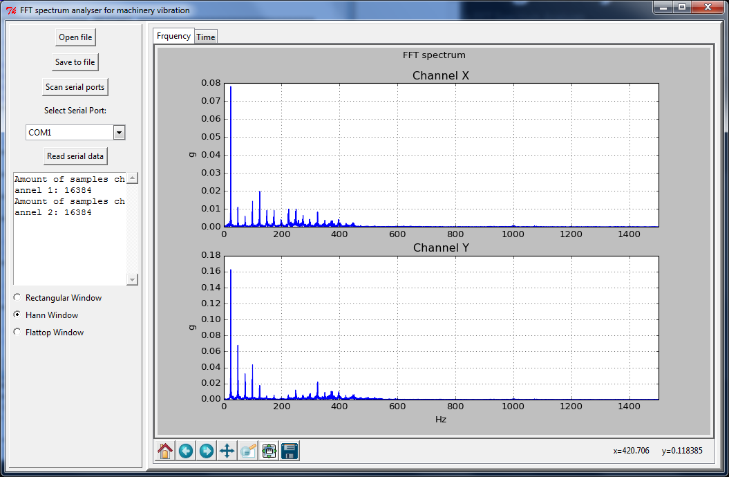
I updated the GUI program, and now it includes the window functions (rectangular, Hann and Flattop). These functions can be selected using radio buttons.

This is a screen shot of the new GUI. The radio buttons are at the end of the left panel.

I also uploaded some text files with acceleration measurements. The file names start with “datos…” and a date and time. These files can be used for testing.

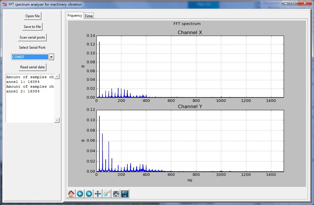
A program with a GUI has been developed (fft_spectrum_gui.py). It uses the Tkinter library, basically because it is the one included with Python, and no additional programs are needed. Also, it integrates very well with matplotlib.

The new program combines the programs acel_file_plot_03.py and serial_avr_01.py. This new interface lets you scan serial ports, select the serial port, save the sampled data to file, and open files with sampled data previously saved. It also has a scrolled textbox where messages are displayed (the ones printed on the previous programs).

A screen shot is shown below.

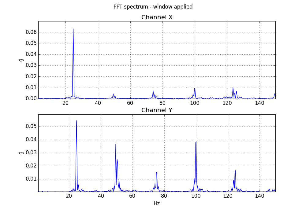
Window functions are used to avoid signal leakage, that can hide low amplitude level signals when their frequency is close to high amplitude level ones. To avoid this leakage, the input samples are multiplied to a mathematical function, so the samples at the center of the sampled time are favored while the values of the samples at the extremes, are lowered. Usually Hann and Flattop windows are applied. Using Python and Scipy, applying window functions is very simple.

First, you have to import the signal module

from scipy import signal

Then create the window function coefficients. For the Hann window use

w = signal.hann(N, sym=False)

For the Flattop window use

w = signal.flattop(N, sym=False)

N is the length of the signal (number of samples).

Finally apply the FFT to the signal weighted with the window function.

yf = fftpack.fft(y*w)

Program acel_file_plot_win_01.py plots the FFT spectrum using the window functions.

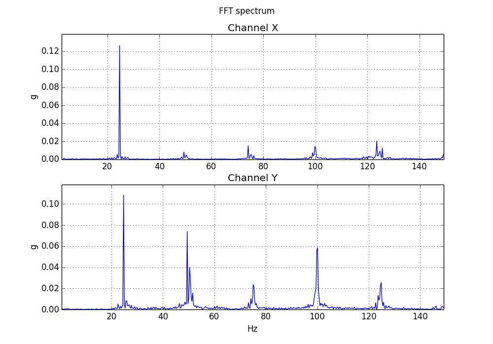
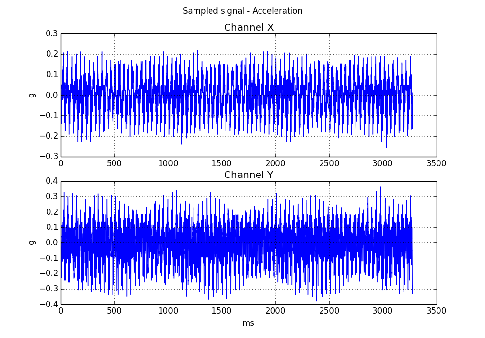
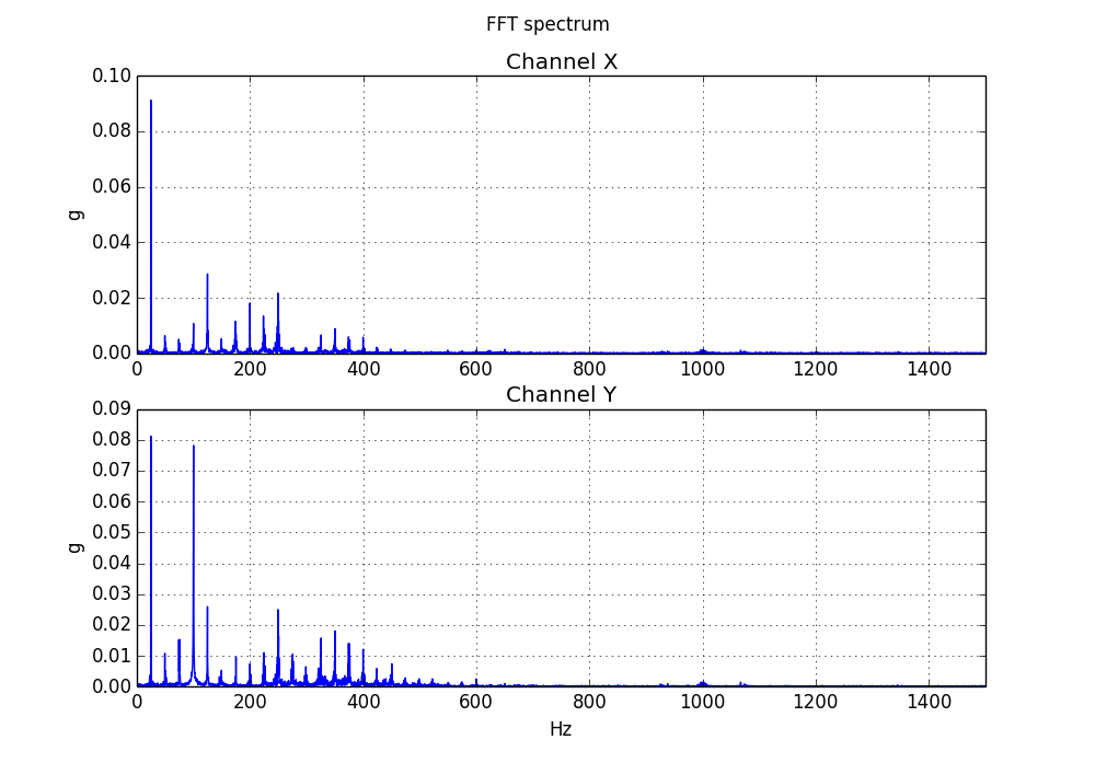
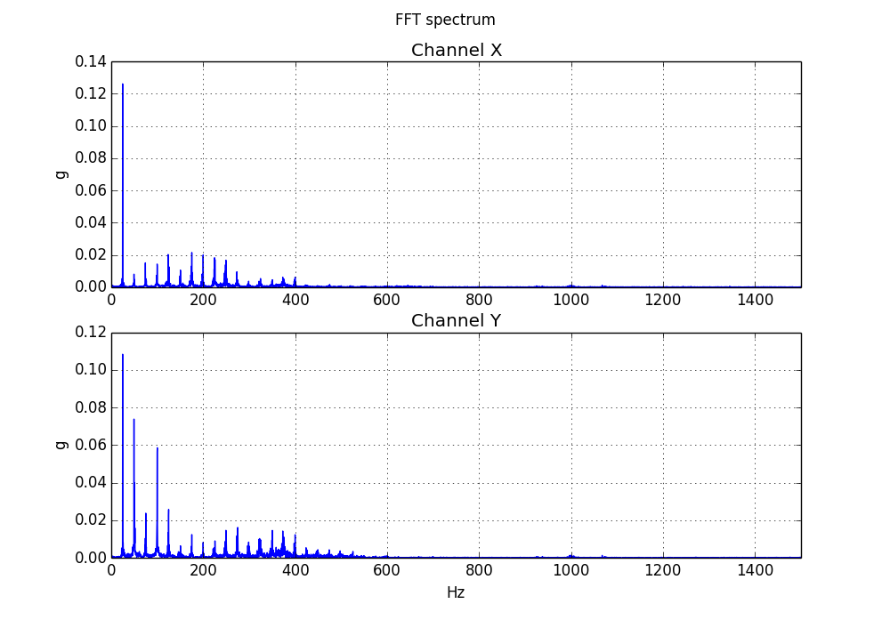
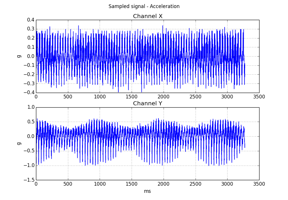
After applying the window functions, no much change is visible in the signal frequency separation and only the amplitude is reduced. Apparently, signal leakage is low for the sampled data used, and further testing would be required to validate this functions.

Three measurements on the same rotating machine were taken for testing the instrument response. The first measurement was taken without modifying the machine.

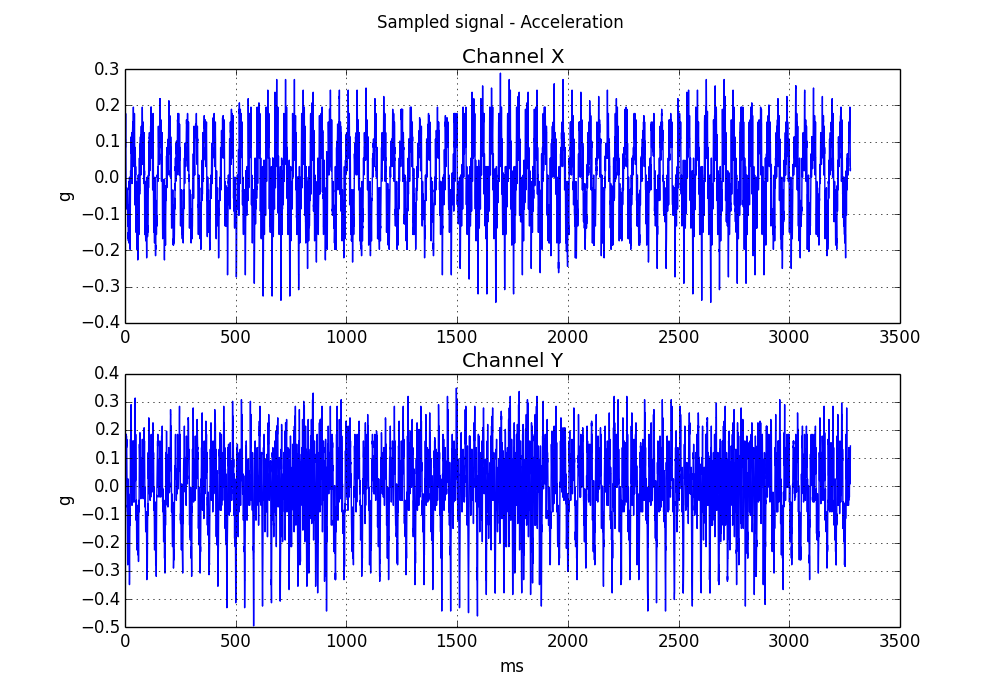
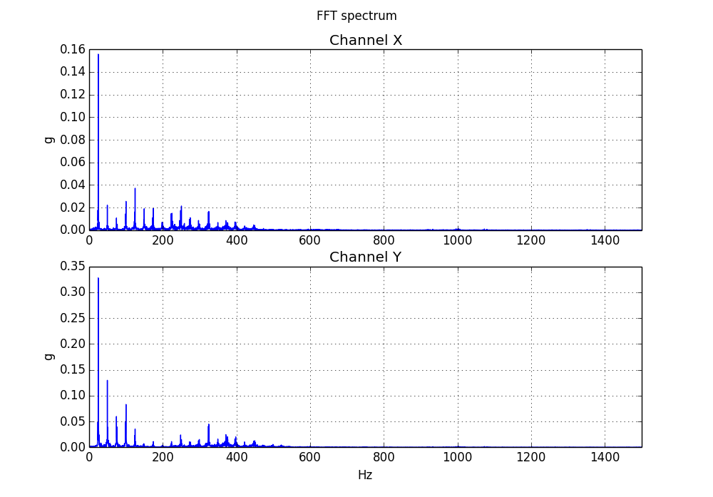
The second test was taken adding weight to a certain place on the machine, for creating an imbalance. It can be clearly seen an increase in the magnitude of the acceleration, both in time domain and frequency domain.

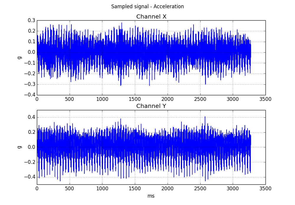
Finally, more weight was added to increase the imbalance and a third measurement was made. Again, an increase in the acceleration amplitude is observed.

The original program was not properly scaled. The signals were plotted using the ADC values and the number of samples obtained.

The signal size has been scaled to g. The ADXL335 has an output from -3g to +3g, for a voltage range from 0 to 3.3 V, that is converted by the ADC to values from 0 to 1023. The original signal is multiplied by 3.0/512, and then the DC offset is determined, taking the average of all the readings. This approach assumes that the average value of the vibration signal is 0.

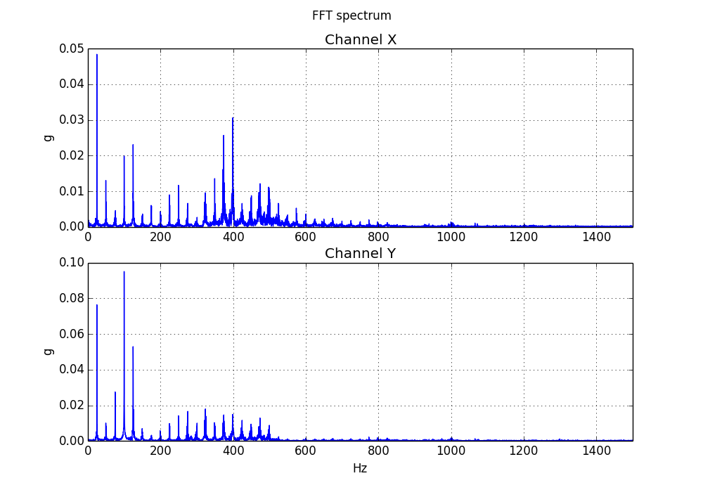
A correction to the time scale has also been done, considering the sampling rate and the number of samples taken. Frequency range has been limited to 1500 Hz, the maximum frequency that the ADXL335 con provide on the X and Y axes.

The corrected program is acel_file_plot_03.py, and the resulting plots are now properly scaled.

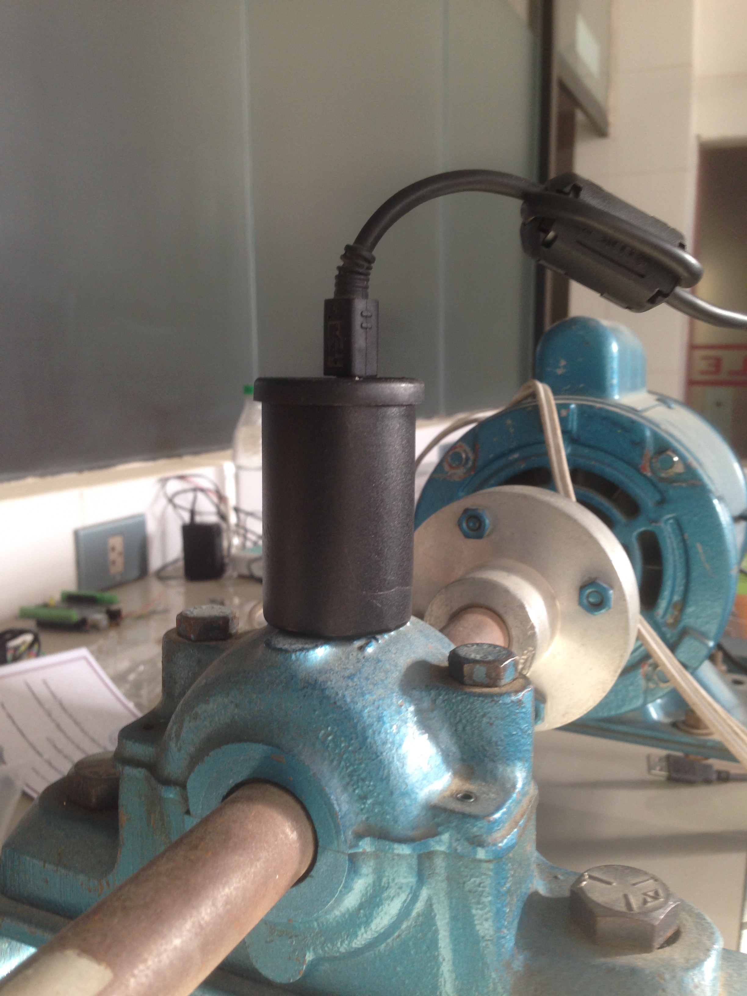
The accelerometer and the Arduino Nano fit together inside a plastic probe (camera film canister). A strong magnet is also included inside, so the probe can be attached very firmly to different parts of a rotating machine and measure its vibration.

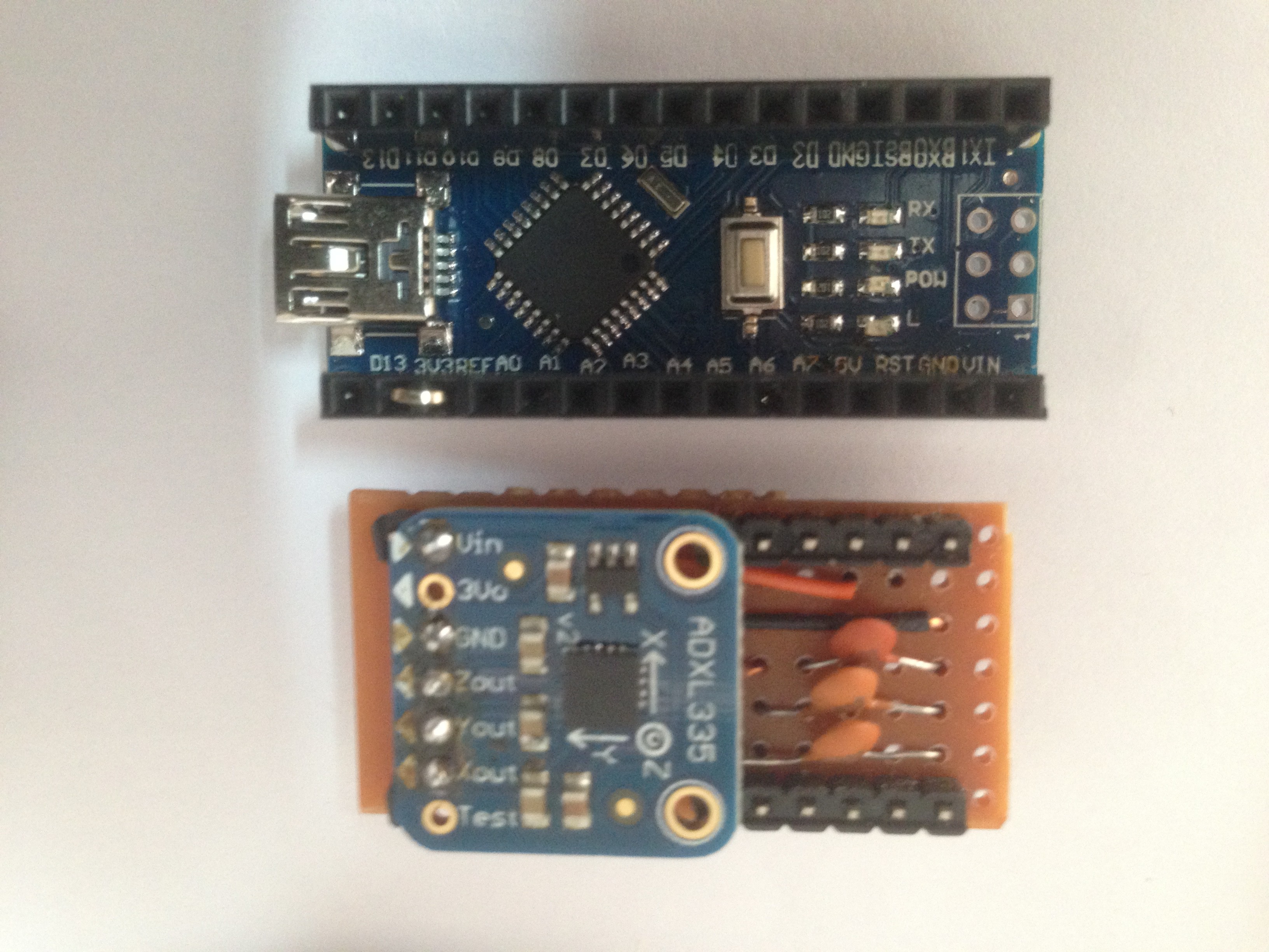
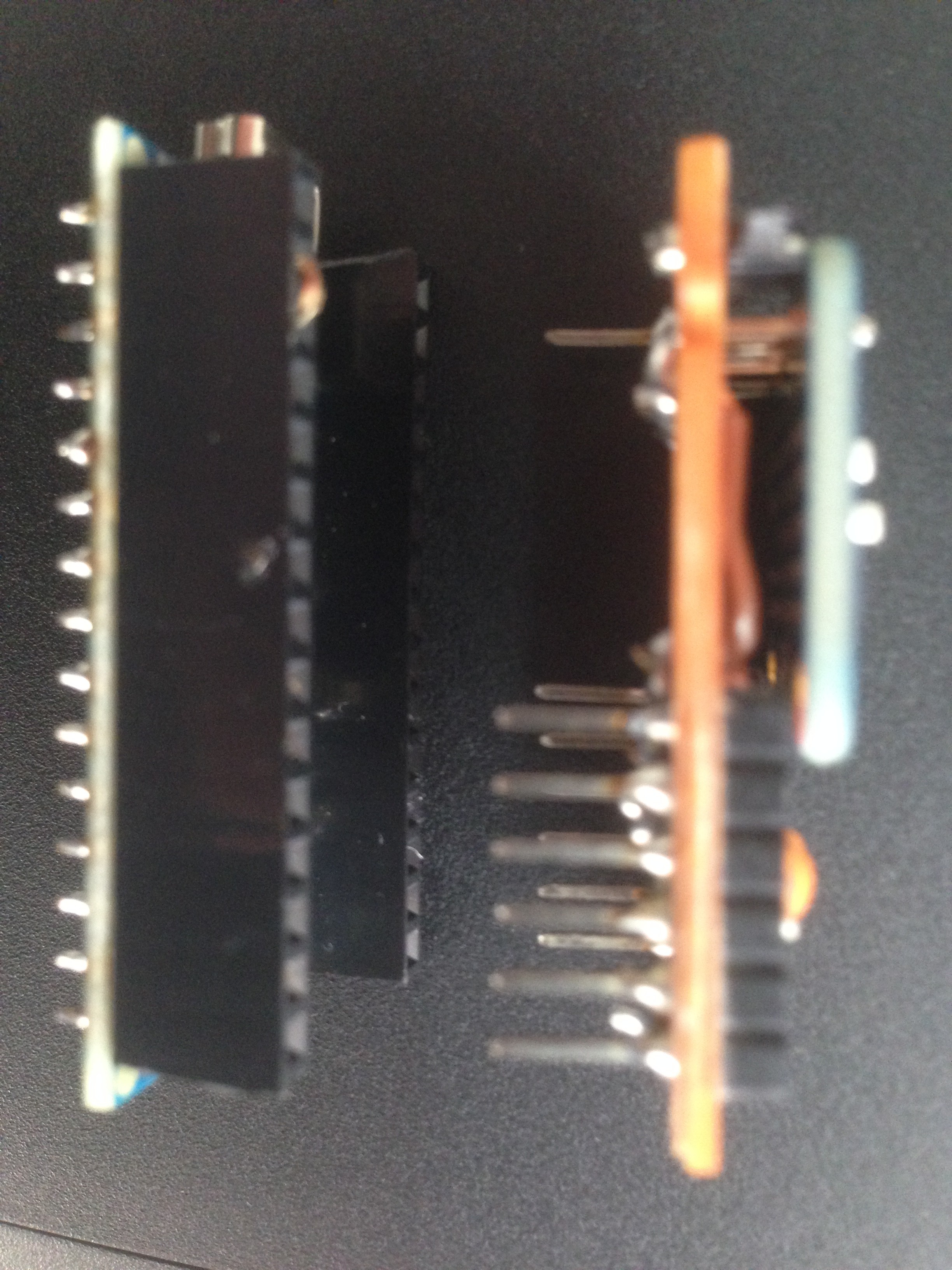
The accelerometer breakout board is soldered to a perforated board and three capacitors are connected and soldered, one to every analog output form the ADXL335. Header pins are placed at the sides of the board and arranged so this pins fit inside single line sockets soldered on the Arduino Nano, instead of the regular connector headers.