Ted Yapo
-
DAC Impulse Responses
05/15/2018 at 23:26 • 0 commentsI wanted to copy these figures from the Maxim application note, but they're copyrighted and whatnot, so I wrote some quick python to calculate Fourier transforms for piecewise-constant functions and drew my own. I would have paid good money for access to something like this when I took those undergrad courses...
![]()
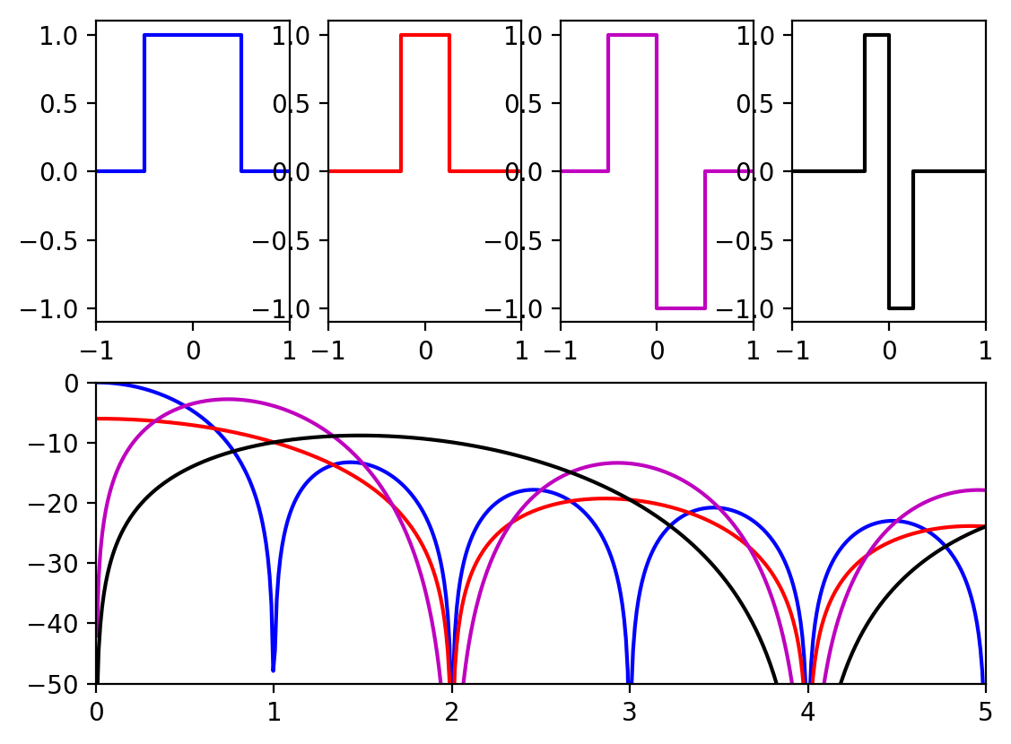
Along the top are the four DAC impulse responses supported in the MAX5879, and in the bottom plot are the corresponding output envelopes in dB vs frequency (1 = the sampling frequency, so the first Nyquist zone extends from 0 to 0.5).
The first response (blue) is the familiar zero-order-hold, which just outputs a constant value during each sample period. This is the response implemented in the FL2000 chip. You can see that the output spectrum has zeros at multiples of the sampling frequency.
The second response (red) drops back to zero (known as return-to-zero) for half the sample period. This results in an output envelope that has zeros at even multiples of the sampling frequency. This is beginning to approach the ideal of an infinitely narrow output sample, which would have a flat output spectrum.
The third response (magenta) inverts the output for half the cycle. This has a zero at DC, so is only useful for RF generation, not baseband signals, but has a higher envelope in certain Nyquist zones.
The last response (black) also inverts but returns to zero for half the period.
You can see how choosing one of these outputs from the DAC could really come in handy when using higher-order Nyquist zones: you can tailor the output envelope for the frequency you want to create.
One of the goals of this project is to create a simple, cheap add-on to the FL2k dongles to modify this response and allow better generation of higher frequencies.
Oh, I guess I'll drop the code that generates the figure here. It's a one-off, so it ain't pretty, but it works:
#!/usr/bin/env python import numpy as np import matplotlib.pyplot as plt t0 = np.array([-2, -1, -1, 1, 1, 2])*0.5 h0 = np.array([ 0, 0, 1, 1, 0, 0]) t1 = np.array([-4, -1, -1, 1, 1, 4])*0.25 h1 = np.array([ 0, 0, 1, 1, 0, 0]) t2 = np.array([-2, -1, -1, 0, 0, 1, 1, 2])*0.5 h2 = np.array([ 0, 0, 1, 1, -1, -1, 0, 0]) t3 = np.array([-4, -1, -1, 0, 0, 1, 1, 4])*0.25 h3 = np.array([ 0, 0, 1, 1, -1, -1, 0, 0]) fmax = 5 n_points = 1000 def plot_pair(t, h, style): f = np.linspace(-fmax, fmax, n_points) H = np.zeros(n_points, dtype=complex) # calculate Fourier transform H(f) for piecewise-constant function h(t) for i in range(1, len(t)): H -= h[i] * (np.exp(1j*2*np.pi*f*t[i])/(1j*2*np.pi*f) - np.exp(1j*2*np.pi*f*t[i-1])/(1j*2*np.pi*f)) plt.plot(t, h, style) plt.axis([-1, 1, -1.1, 1.1]) plt.subplot(2, 1, 2) plt.plot(f, 20*np.log10(np.abs(H)), style) #plt.plot(f, np.square(np.abs(H)), style) plt.subplot(2, 4, 1) plot_pair(t0, h0, 'b') plt.subplot(2, 4, 2) plot_pair(t1, h1, 'r') plt.subplot(2, 4, 3) plot_pair(t2, h2, 'm') plt.subplot(2, 4, 4) plot_pair(t3, h3, 'k') plt.axis([0, 5, -50, 0]) #plt.show() plt.savefig('DAC_impulse_response.png', bbox_inches='tight', dpi=200) -
Interpolating with transmission line?
05/15/2018 at 04:33 • 4 commentsSo, I started playing around with transmission line models for generating short sampling pulses, and it occurred to me that you could use a transmission line to interpolate between DAC samples. It's kind of like doubling the sample rate just using a piece of wire! Here's a circuit I've been playing with:
![]()
The circuit is amazingly simple. The voltage source and 50-ohm resistor model the FL2k DAC (with impedance-matching network to have 50-ohm output, like on the breakout PCB). The only other element in the circuit is a 50-ohm transmission line cut to have a 2.5ns delay (the delay must be one quarter of the sample period). This line is literally just a piece of coax open at one end. The circuit works by taking advantage of the signal reflection from the unterminated end of the transmission line.
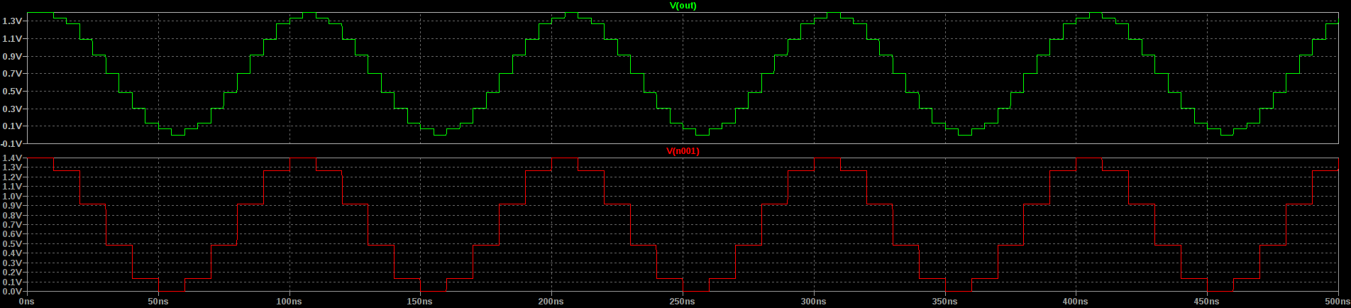
Here are the input and output waveforms from the simulation:
![]()
The bottom (red) trace is the input. I've simulated a 100 MSPS DAC generating a 10 MHz signal (that's the equation controlling the behavioral voltage source). The top (green) trace is the output of the circuit, which shows that another sample point has been interpolated between each pair of input values, which could be mistaken for doubling the sample rate.
How does it work?
The unterminated end of the transmission line causes a reflection of each step in the input voltage from the DAC. Since the reflection must travel the line both ways, it takes 5ns for the reflection of a DAC step to get back to the summing point where the output is taken. This 5ns is half of the sample period, so the DAC by now is half way through the next sample. Summed with the reflection of the previous sample, this creates an interpolated point which is the average of the two adjacent samples.
Is it practical?
I don't know yet. It's too late tonight to get this up and running in hardware. I'll have to try it as soon as I get a chance. In simulation, anyway, it certainly looks interesting.
Just to be clear, there aren't twice as many "real" samples being generated; the Nyquist rate for this system is still 50 MHz even though there are essentially 200 MSPS being output.
At this time of night, I'm not even entirely sure what this achieves, but I can figure that out tomorrow.
EDIT: I can't sleep.
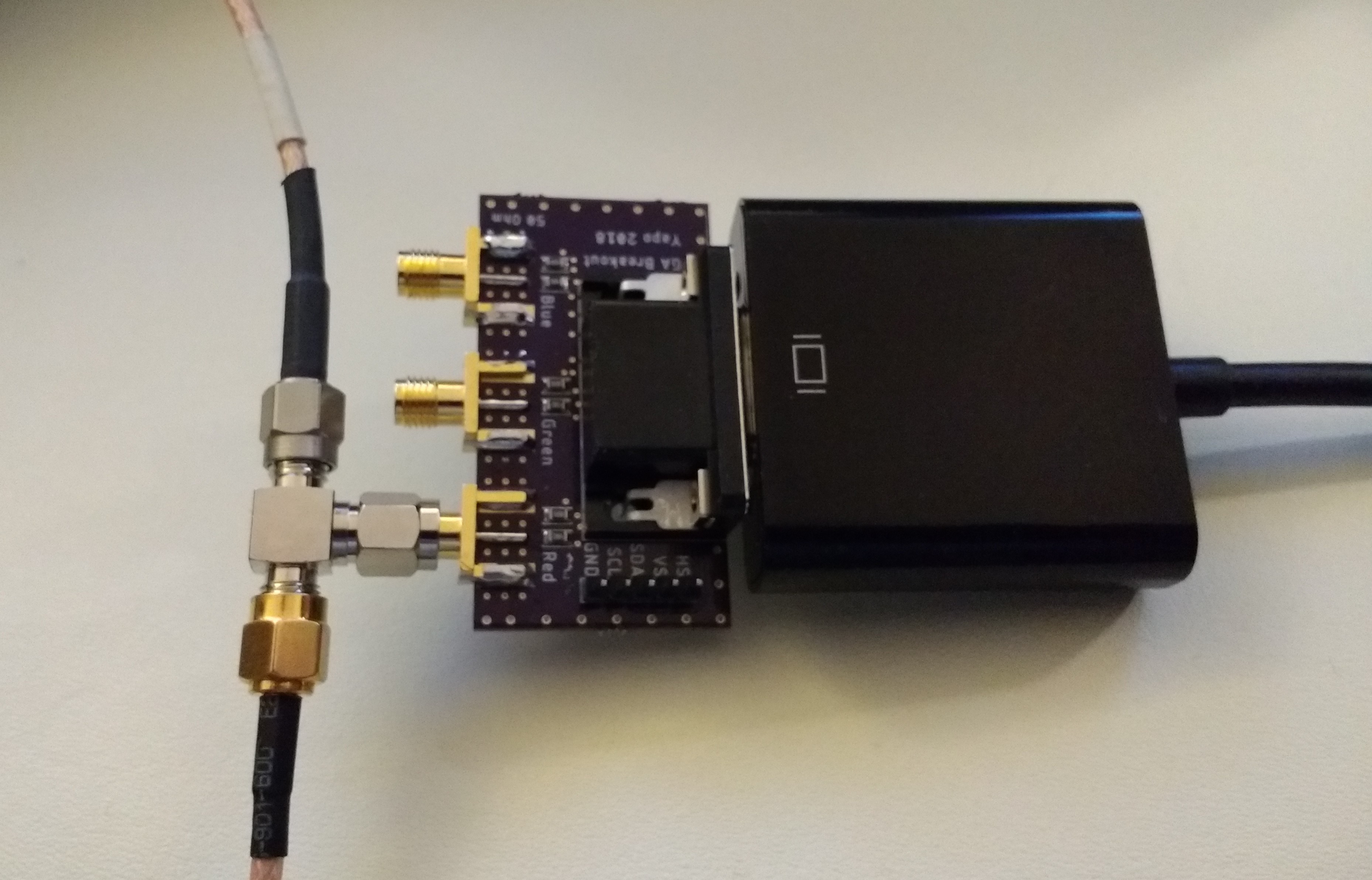
I just had to try it out. I used an SMA T-connector to add the unterminated line to the output of the FL2k dongle (the other line goes to the oscilloscope).
![]()
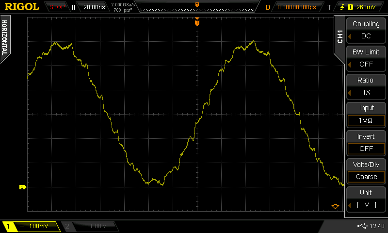
To test it, I generated a 6.4 MHz signal using an 80 MHz sample rate (about the fastest I can do through my USB 3.0 hub). With no line connected to the T, the output clearly shows the 12.5 ns sample periods:
![]()
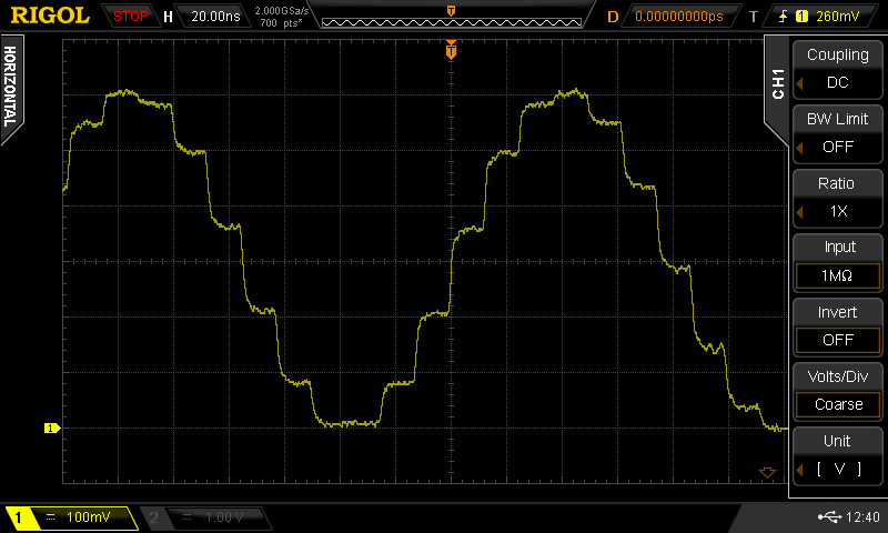
After connecting a line of around the right length, you get this waveform:
![]()
it certainly looks like it's doing something. Hopefully this will be enough to allow me to sleep, and I can look with the spectrum analyzer tomorrow...
-
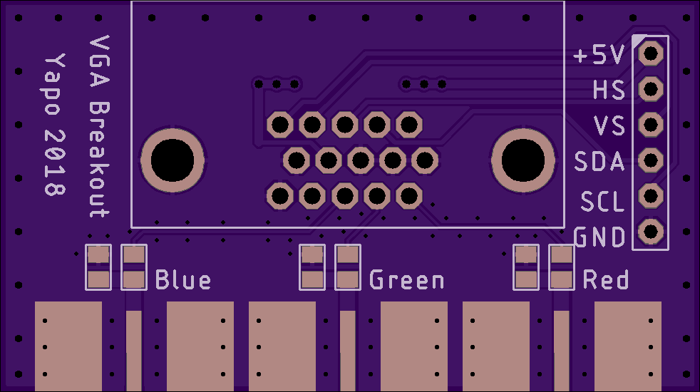
Updated Breakout PCB (again!)
05/15/2018 at 01:36 • 0 commentsI modified the breakout PCB to include the +5V line, which I had overlooked before. The FL2k dongles, at least the ones I have, do supply 5V on this line. The latest design is in the GitHub repo, and the PCB is shared on OSH Park.
![]()
I think this is the last iteration. Probably :-)
FL2k Experiments
Exploring the FL2k USB-to-VGA dongle for signal generation