It has been more than one month since our last hackaday update. The Kalman filter and the PID were the obstacles that stopped us, which our team had very little knowledge of. In general, we took a step forward with the grid system we proposed and implemented task assignment, auto-routing, collision avoidance, as well as error correction with PID on the system. To make the framework more comprehensive, we also implemented a simulation platform featuring all functions implemented on the real robot. The following post will discuss updates discussed above respectively.
Task Assignment
We found that the original framework we developed (please refer to log ) was naive and not efficient. It would be better if robots can sort out their target destinations before they are on the move. With suggestions from various professors, we began digging into academia, trying to find existing algorithms to tackle the problem. It didn’t take us long to find that the task assignment among multiple robots is similar to the Multiple Travelling Salesman Problem, which is a variation of the (Single) Travelling Salesman Problem and is NP-hard. Most of the optimal algorithms are beyond our scope of understanding. Then we began looking for algorithms that produce suboptimal results and are easier to implement. The one algorithm that we implemented was the decentralized cooperative auction based on random bid generators. I will briefly explain this algorithm below.
At the very beginning, each robot would receive an array of destinations to go to and would calculate the closest destination relative to their current positions. There is a synchronized random number generator among all robots. Before every round of the bidding, all robots would run this number generator, which outputs none-overlapping numbers between 1 and the total number of robots in the system for each robot. Having generated the number, robots would bid in turn based on the random number they got. When it is one robot’s turn to bid, it would broadcast its bid and its cost among all robots. Robots haven’t yet made the bid needed to process the bid made by other robots. If this bid coincides with its own pending bid, it needs to delete this current bid and reselect the next closest, available destination. The robots need to do this auction for m times, each time one robot would have a different random ID (thus would make bids at different orders). In the end, robots would unanimously pick the round of bidding with the least total distance.
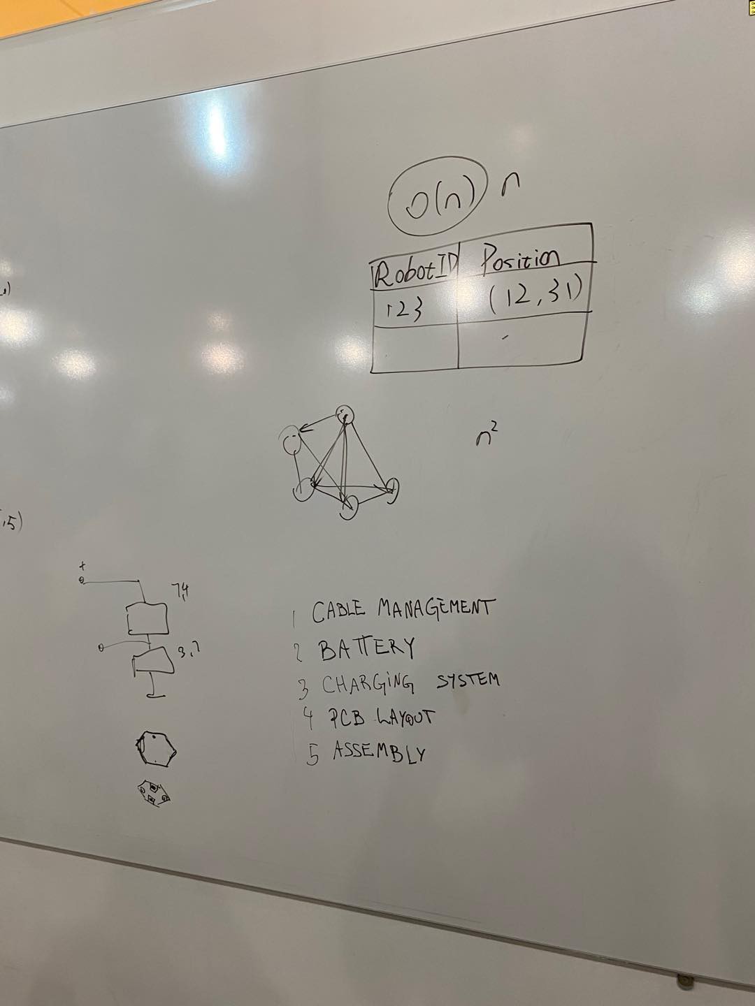
Suppose the size of the task is n, the robots are programmed to do m rounds of auction to find the smallest total distance, the time complexity to produce a suboptimal assignment is only O(mn). This is a much lower complexity than the optimal algorithm that needs factorial time.
Due to the time constraint, we could only implement a simplified version of the algorithm, where the auction would only last for one round.
Figure 1. FLow chart of task assignment
Auto-routing
In a grid system, routing from point A to point B (not considering collision) is easy. We defined the length of each cell in our grid as 30cm; the origin is at the top left corner of the grid, the x coordinate increases as going to the right of the grid, while the y coordinate increases as going to the bottom of the grid. Please refer to figure x for further details of our grid setup. To get from point A to point B, the robot only needs to calculate the differences in x coordinates and y coordinates. The intermediate waypoint would have the same x coordinate as the starting point and the same y coordinate as the destination point.
Figure 2. Grid setup
Yet this brute-force way of routing may lead to collisions at various intersections. In a grid system, collisions occur because more than one robot is about to occupy the same coordinate at the same time. Thus, we assumed collisions could be avoided by dispersing the routes of all robots and making them occupy different coordinates at the same time. In academia, there exists many centralized and decentralized solutions for planning collision-free routes. But due to time constraints, the routing we implemented was just a variation of the brute-force way mentioned above. To sufficiently disperse robots’ routes, we exploited the property of the grid system. Suppose a robot needs to get from point A to point B, and the differences in x coordinates and y coordinates are m and n respectively. There would be in total ((m + n) * (m + n - 1) * … * n / n!) many different routes. Based on this knowledge, our auto-routing function generates four waypoints instead of three. The two middle waypoints have random x coordinate values between starting and finishing points.
Collision Avoidance
Despite our effort to implement the collision-free routing function, in practice we still observed frequent collisions among robots. A collision avoidance system based on infrared thus became necessary. Based on other researches, we classified possible collision scenarios in our system as head-to-head collision and intersection collision. Both these two cases have subcases, which are discussed in the figure below.
Figure 3. Classification of collisions
As described in the hardware part above, the infrared receivers and emitters are arranged in a certain pattern. Such a pattern allows robots to detect infrared signals coming from front, left and right. Robots would send infrared signals in a pulsatile manner, where the emitter would be on for 1ms and off for 20ms. Robots use 12-bit analogread to read infrared signals from receivers. The reading ranges from 0 to 4095. The reading has a threshold value, once a reading gets above the threshold, the robot would consider a possible collision from the direction of the receiver that has this reading and output a one.
Based on the readings from the six receivers, we drafted a simple protocol to avoid the collision scenarios mentioned above. Rules are as follow:
1. If a robot receives infrared signal at the front (receiver 3), it would reroute and turn left to avoid the collision from the front.
2. If a robot receives infrared signal at the left (receiver 1 and 2), it would not act.
3. If a robot receives infrared signal at the right (receiver 4 and 5), it would start a random timer. Once the timer expires and no message was received, it would broadcast a message including its ID, current direction, current coordinates.
The order of priority of the collision scenarios is the same as the order above, where the head-to-head collision has the highest priority, then the intersection collision. Inspired by the real-world traffic rules, we determined that at an intersection, the other vehicle coming from the right relative to self has higher priority. In our case, in order to avoid two robots sending out messages simultaneously at an intersection, the vehicle relatively coming from the left would initiate the communication.
Once other robots in the system have received the collision message from case 3, they would compare this coordinate with its current route and try to calculate the collision coordinates between self and other, where the routes of two robots would intersect. If the collision coordinate is both on self and the other robot’s route, this robot would calculate their distances to the collision coordinates respectively. If self is closer to the coordinates, the program would output action 0 for self and action 1 for other, where self would carry on with its task and the other robot needs to stop and wait, vice versa. The action for the other robot, together with the other robot’s ID and the collision coordinate would be broadcast to the rest of the swarm. The initiator would act according to the action given by its peer. For the robot that needs to move along the current route, once it has gone past the collision coordinate, it would broadcast another message indicating it has passed the collision coordinates, so that its peer that stopped could start moving again. The process is similar to computer networking protocol that consists of SYN, SYN/ACK, ACK.
Figure 4. Flow chart for initiator
Figure 5. Flow chart for receiver
Error Correction
It’s important to keep robots running on the grid we constructed. If robots go off-course frequently, the auto-routing functions we wrote would be wasteful, and there would be more possible collision scenarios than we classified earlier. This would drastically complicate the collision avoidance scenarios. There are two reasons behind robots going off-course, first is when robots’ directions are not aligned with north, south, west or east after it turned, second is when robots are going forward, two wheels are not turning at the exact same speed.
PID is one solution to both of the problems. We implemented two PID systems on our robot, one for turning and one for going straight. We only used Kp in both PID systems. In the PID for turning, turning speed is proportional to error. Robot acquires the error locally through the difference between the current encoder ticks and the target encoder ticks (target encoder ticks represent the number of encoder ticks needed to turn a certain angle).
speed = kp * error
Another PID is for bringing an off-course robot back to its course. The robot calculates the error by comparing the absolute coordinate it receives from the camera with the current trajectory it is on. Error is positive if the robot is off-course relative to the right, negative if the robot is off-course relative to the left. This error would be sent into another PID function, which would output two different speeds that the program needs to apply to two wheels, in order to bring the robot back on course.
In practice, we found that having 100% trust in either local information (encoder ticks) or global information (absolute position update) would be faulty. For encoders ticks, though interrupt would update encoder ticks almost instantaneously, the data might be very noisy; for absolute position update, it updates at a much lower frequency (once every second), and there would be certain error between the actual position of the robot and the position advertised by the server (since it takes hundreds of milliseconds for the camera to capture the image, analyze the image and send the coordinates into the LAN). To obtain a cleaner, more accurate error value for PID, we need to implement Kalman filters that do the following:
1. Sensor fusion, which fuses the data from encoder ticks, absolute position update, even IMU.
2. Absolute position error corrector, which would calculate the up-to-date absolute position of the robot based on the delayed position update from the camera, as well as current pose estimation.
Yet it was never easy to implement any Kalman filter. The biggest obstacle was understanding the Kalman filter. We don’t have anyone in our team that is familiar with the Kalman filter, so we have to learn it from ground up. This would not be an easy task. The deeper we dug into this field, the more we felt this would be a mission impossible within 1 month. If we were to devote all our energy to implementing the Kalman filter, the research target would drift from researching multi-agent robotic systems to learning inertial navigation. The latter is already a well-established subject and it would be dangerous if we spend too much time on it.
To solve some of the problems above without any Kalman filter, we implemented timers. After the robot turns for a certain degree, it needs to stop and wait for 1 second before decoding the positional data from the server, which guarantees it getting stable and clean data. If the coordinates received from the server have huge errors compared with the local coordinates, the robot would ignore the current update and wait for the next round of update. If the update still has huge errors, the robot needs to believe in it. We couldn’t solve the delay in the global update, so the robot would rely more on their local encoder ticks instead of the global update.
Figure 6. Flow chart of PID
Production of demo
With all functions above implemented, the system is capable of the following task: user inputs desired destinations’ coordinates, server broadcasts these coordinates among robots, robots then self-assign tasks, plan out a path to reach their own target, finally move towards the target while avoiding collisions. The best demo that can be made out of the current task is shape formation. Inspired by the researchers at Northwestern University, we decided to use our robots to lay out the letters, “N”, “Y”, “U”.
Unfortunately, since the functions/algorithms on our robots are still primitive, we couldn’t lay the robots so densely as Northwestern researchers. Instead, we looked at a 5 * 5 matrix to find out which row, column pairs should be taken up to form each letter. We then mapped this row, column pair to the coordinates in the grid system. When executing theshape formation, we first put the robots on the ground randomly, turned them on, then sent the entire set of coordinates needed for this letter.
We started with letter “Y”, since it only needs 7 robots; then letter “U”; at last letter “N”. The process of preparing the demo was not very smooth. Since the collision avoidance functions were still rather primitive, when we were dealing with letters that need more robots, such as “N”, we encountered numerous deadlocks and edge cases not specified in our program. It would be important that we focus on this field of research in future iterations. Despite the difficulties, we still managed to form the letters as we expected. Please check out the time-lapse video down below.
Figure 7. NYU shape formation
Simulation
To better demonstrate our physical field test, we planned to simulate a model that is similar to our real robots in Webots. The first method that came to my mind was that I can simply build a model from scratch using the 3d-modeling functionalities in Webots. As we partly mentioned in the past blog posts, 3d-modeling in Webots is “component-based”. To build a model, we need to create each of its components and assemble them together. In the case of building our robots, we need to create components like wheels, robots’ body parts, various sensors, and etc. (Please refer to Figure 8 for more details). It is interesting to note that if we want to code some functional parts like motors and sensors, we have to use components designated in Webots.
Figure 8. “Component-based” modeling
However, considering that our robots are hexagonal, those functionalities could only enable me to create a robot model in some regular shapes like linear, square, and circle, which is not similar to our physical robots. Therefore, we decided to import our 3d-model file of our real robots into Webots to demonstrate a robot model that is really similar to the real ones. This process is pretty tricky. The format of our 3d-model file is .stl while the needed format by Webots is .proto, which is specially used in Webots. Since we had no idea how to convert .stl to .proto, we dug into investigation of the conversion. We could not simply find an existing online platform that enabled us to complete such a conversion. Luckily, we did find a solution that we could convert .stl to .proto with the help of “xacro” language in ROS. Along with the .stl file, we needed to create a new .xacro file, which is used to define the model in .stl file in its shape, mass, core, and etc. After we had those two files needed, we used a python module named “urdf2webots” to convert those two files into a .proto file, which can be imported into Webots.
After we successfully imported our 3d-model, we created other components like motors, wheels, and sensors using the basic nodes in Webots and assembled them together. As mentioned above, using the basic nodes in Webots is to help us better code them, for example, code the motors and wheels to make the robots move. To this stage, our simulation robots seemed pretty similar in shape and size to our real ones. However, the color and texture are distinct because these two features require a lot of texture files to add onto the robot model. Since those files are difficult to obtain and unlike the shape and structure of the robots, such appearance can hardly affect our test result, we chose to ignore the color and texture of our robot model in Webots.
Below are three pictures that can demonstrate our models.
From top to bottom: our first model that was made merely by the basic nodes in Webots; our current model that is created by combining basic nodes in Webots and our imported 3d-model together; our real robot model.
We adapted our real code onto Webots robot controller after we finished building our robot model. As we mentioned above, we have functions including task assignment, auto routing, collision avoidance, and error correction. By simulating and running many tests on Webots, we found out that both task assignment and auto routing work very well on Webots, which is very similar to our physical test. All the robots are able to process the data given by the server and decide its path to its desired destination. (Below is a picture to display the result of one test. This test is to let the robots form a pentagon, where the robots will receive the five points of the pentagon and decide where to go).
Figure 9. Robots form a pentagon
As for the error correction part, we still need to implement PID in the simulation even if we do not have to worry about the technical defects of the robots’ components in real life. In other words, robots in simulation will also go off-course either when moving straight or turning, but just for a different reason. The reason is that in Webots we can not program robots to specify a movement, either forward or turn, in a certain amount of distance or degree. Since we only know the speed of its forwarding or turning, we chose to use time to control the distance and degree. However, this method will cause small errors each time the robots conduct a movement because the rotational motors of the robots can never stop right on time, so they will rotate either more or less than expected. The implementation of PID control greatly reduced the cumulative caused by such small errors. It helps us minimize the error to about 3 millimeters in both x-axis and y-axis. Considering the size of our robots which is around 10 centimeters in length, 10 centimeters in width, and 8 centimeters in height, such an error is very small.
As for the error correction part, we still need to implement PID in the simulation even if we do not have to worry about the technical defects of the robots’ components in real life. In other words, robots in simulation will also go off-course either when moving straight or turning, but just for a different reason. The reason is that in Webots we can not program robots to specify a movement, either forward or turn, in a certain amount of distance or degree. Since we only know the speed of its forwarding or turning, we chose to use time to control the distance and degree. However, this method will cause small errors each time the robots conduct a movement because the rotational motors of the robots can never stop right on time, so they will rotate either more or less than expected. The implementation of PID control greatly reduces the cumulative caused by such small errors. It helps us minimize the error to about 3 millimeters in both x-axis and y-axis. Considering the size of our robots which is around 10 centimeters in length, 10 centimeters in width, and 8 centimeters in height, such an error is very small.
Figure 10. Distance sensors in Webots
Another major obstacle is that the distance sensors in Webots can only detect “Solid”, which is a property of the components in Webots. Generally speaking, many of the basic nodes in Webots have such Solid property, like the motors, wheels, sensors, and etc. In other words, they can be detected by the distance sensor. However, since the body part of our current robot model is imported and is not a basic node, it doesn’t have the Solid property, so it can not be detected by the distance sensor (we did research in the API Functions of Webots to come up with this conclusion). To cope with this issue, we manually added four “borders” onto the robots using the basic node in Webots called “Shape”, which is displayed in yellow in the Figure X + 7 below. We adjust its length, width, and height to enable distance sensors to detect it better.
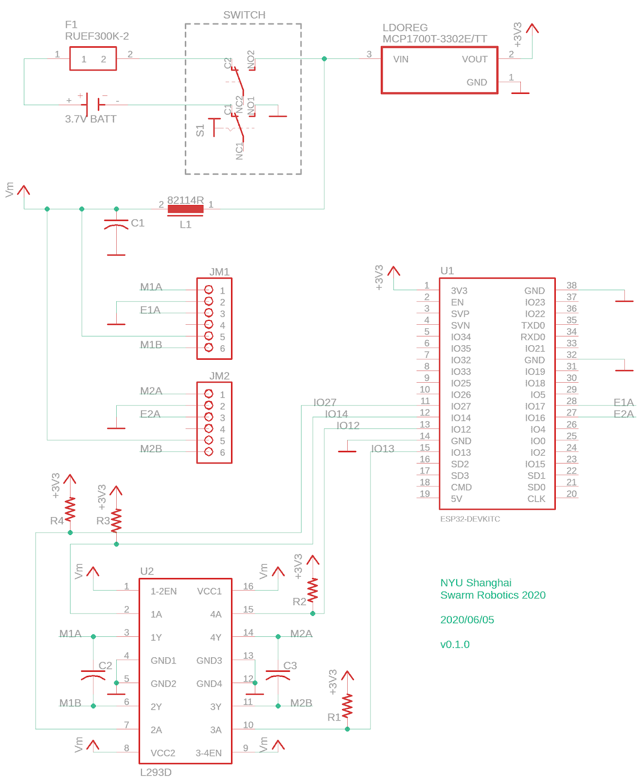
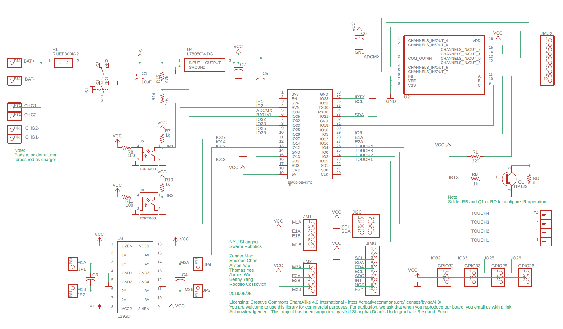
It has been a month since we last updated the details of our project on Hackaday. Accordingly, several hardware tests and hardware changes had ensued. At the end of the last hardware update, we were hoping to finalize PCB v1.0.2 and we did in the week of July 5. For the most part, we concentrated on component placement, minimizing the number of vias across the board and ensuring no vias under the ESP32 module. As for the malfunctioning IMU, we believe it was due to a short circuit induced between the wireless charging receiver coil and the esp32 as both are on the bottom of the pcb. A lot of small adjustments were made on the board and we hoped this version could be a relatively stable one.
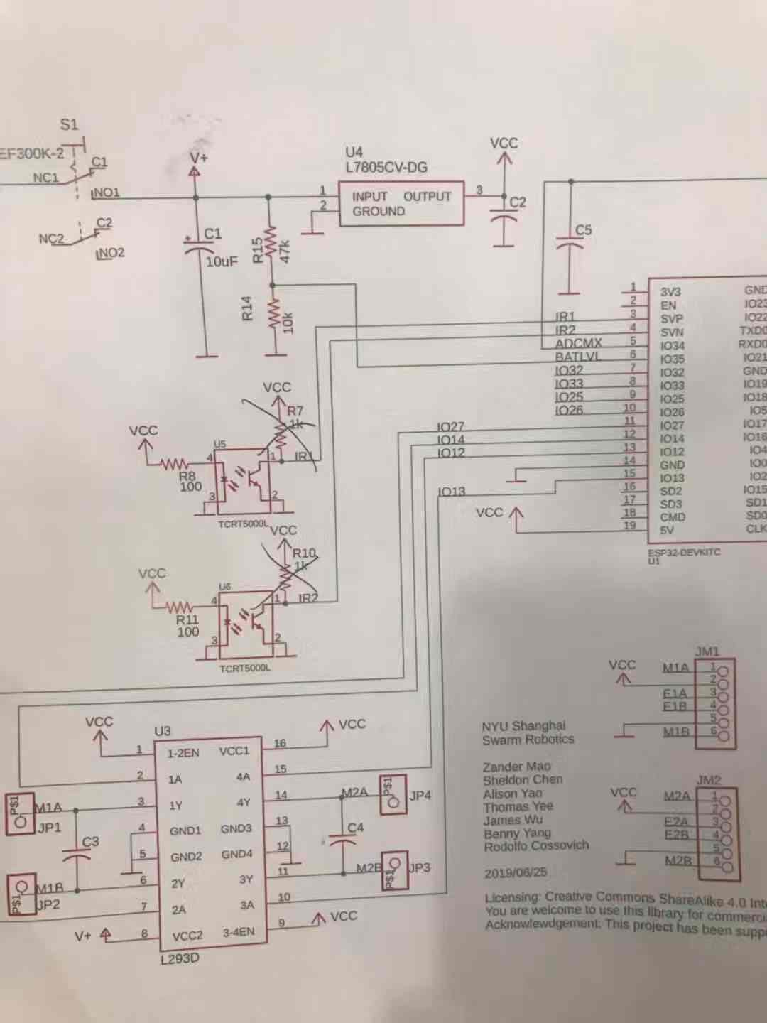
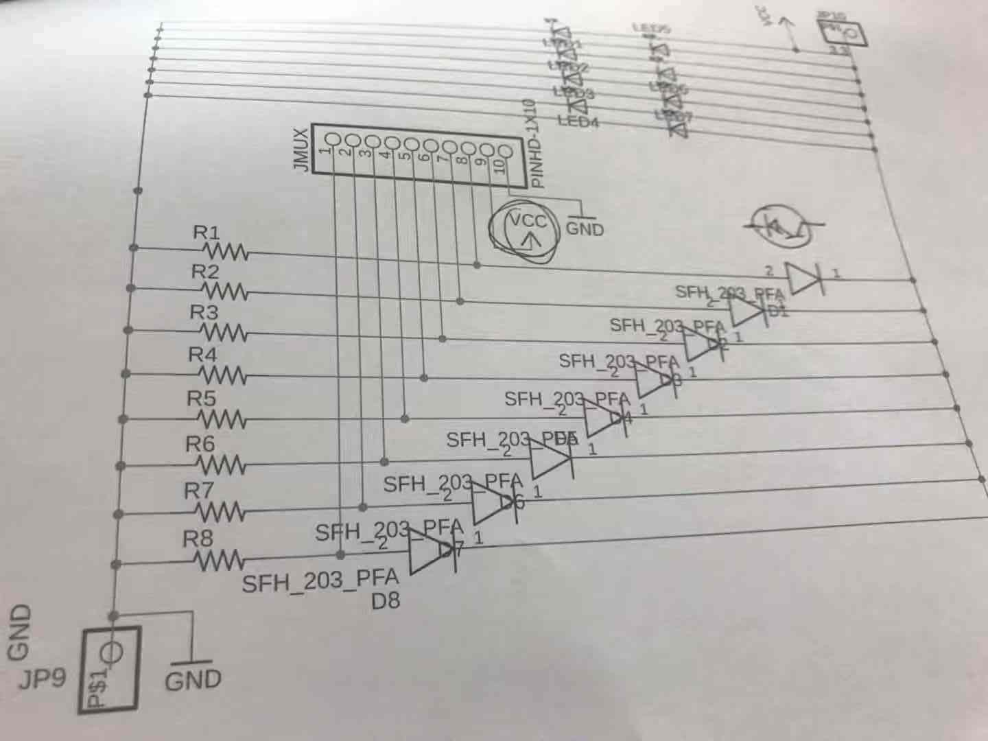
Figure 1. Schematic v1.0.2
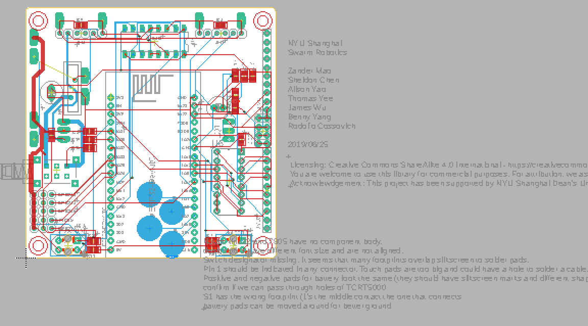
Figure 2. Board Layout v1.0.2
We ran some tests on how long the robot can run with a fully charged battery (with WIFI, motors, LED running). The result was nearly 5 hours every time which is adequate for our robot.
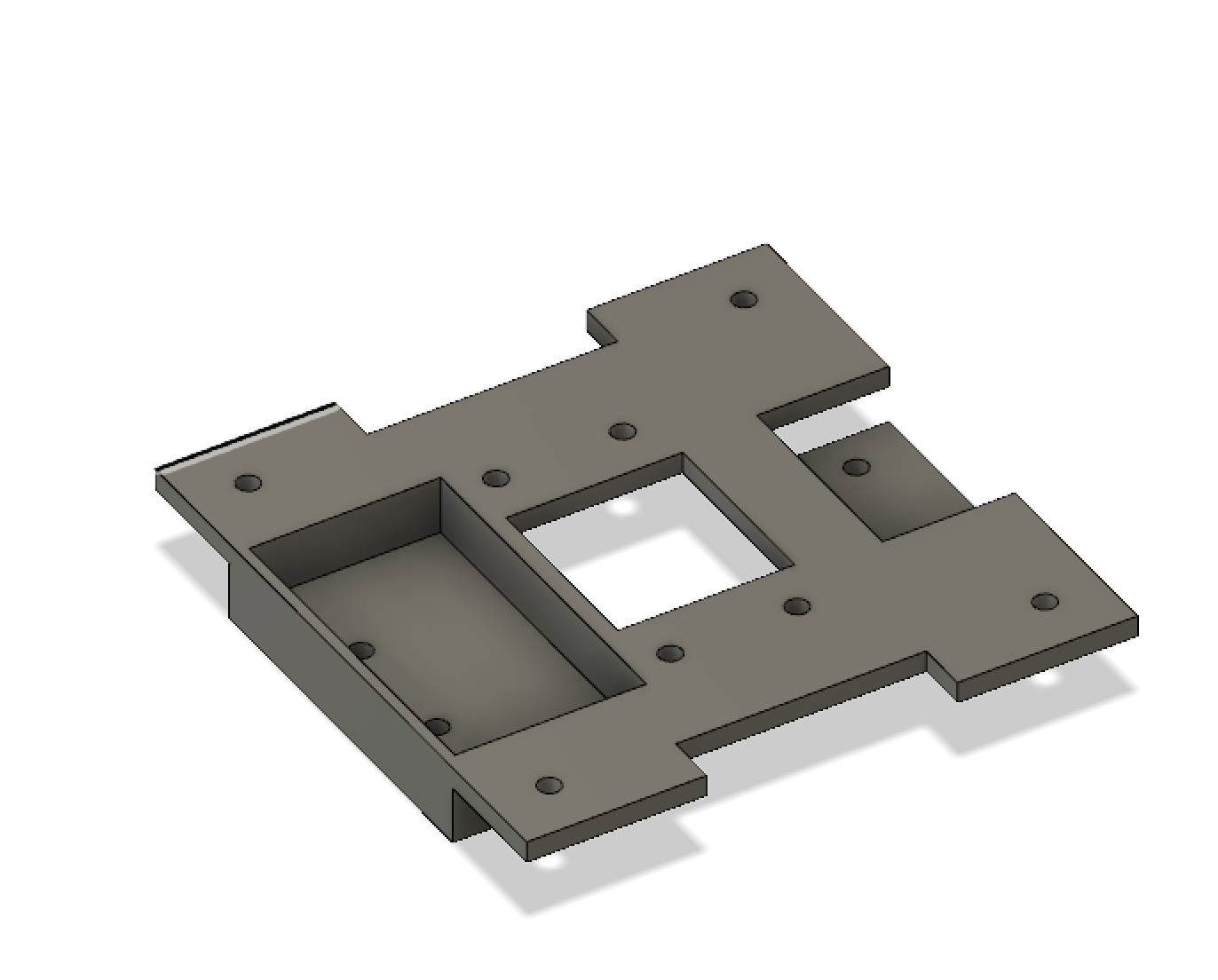
We came up with an idea for the placement of the wireless charging receiver on the robot. The following (figure 3) is a 3D model of the receiver holder that will be attached to the bottom of the robot. Ideally, the receiver will be attached to the holder and as the robot moves to a flat charging spot, the battery will then be charged. Therefore, the distance between the receiver and the transmitter is important. The recommended distance is between 2mm to 8mm.
Figure 3. Receiver plate design
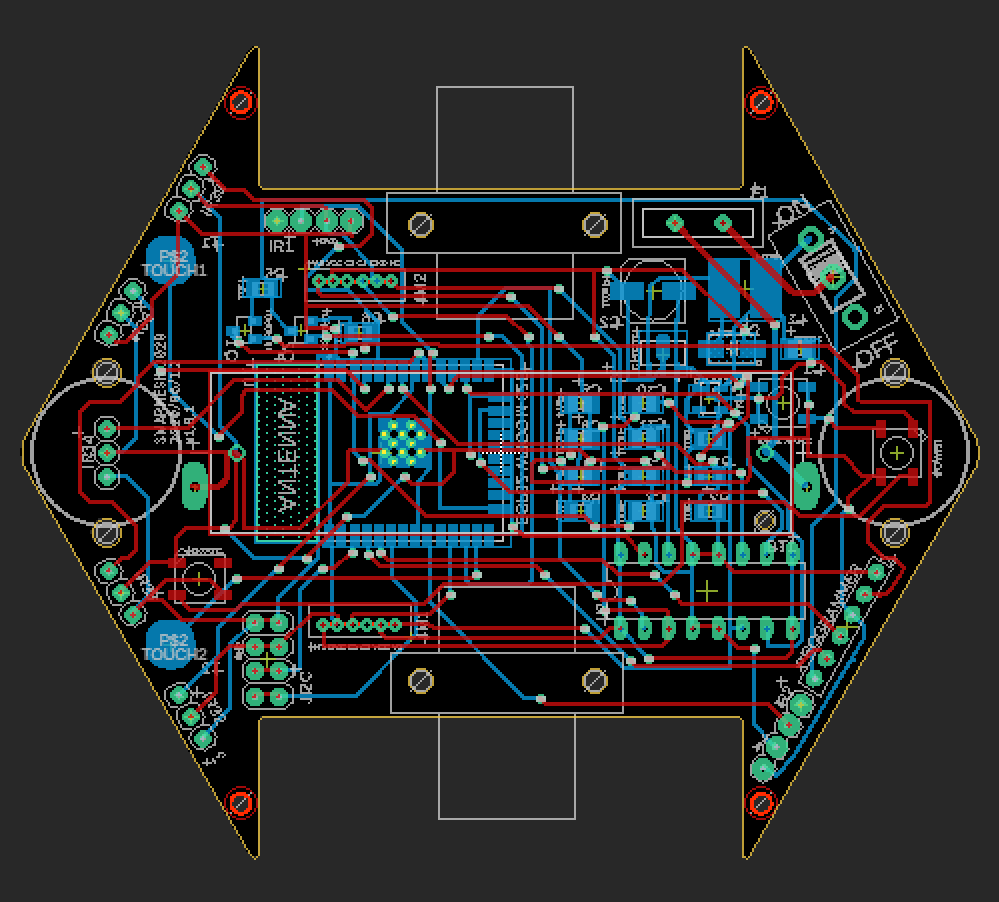
Once we made all the adjustments, we sent PCB v.1.0.2 for manufacturing. Figure 4 is an image of the bottom of PCB v1.0.2. The greatest weakness in this board was the infrared sensors placed at the front of the robot. Other than this, the approximate positions of all other components remained consistent with our final design. The two rows of 6 pins on the PCB are for serial communication, and we decided to use the Ai Thinker USB TO TTL programmer (Figure 5). It was a reliable product, and as expected, we were not disappointed by its performance and consistency. The reset button also worked well (looking back, it was smart to add it). The holes for the switch came out a little too large, which caused some problems in switching on the robot, but in a later version, we fixed this problem. The location of the RGB LEDs was satisfactory.
Figure 4. Bottom view of PCB v.1.0.2 Figure 5. Ai Thinker USB TO TTL Programmer
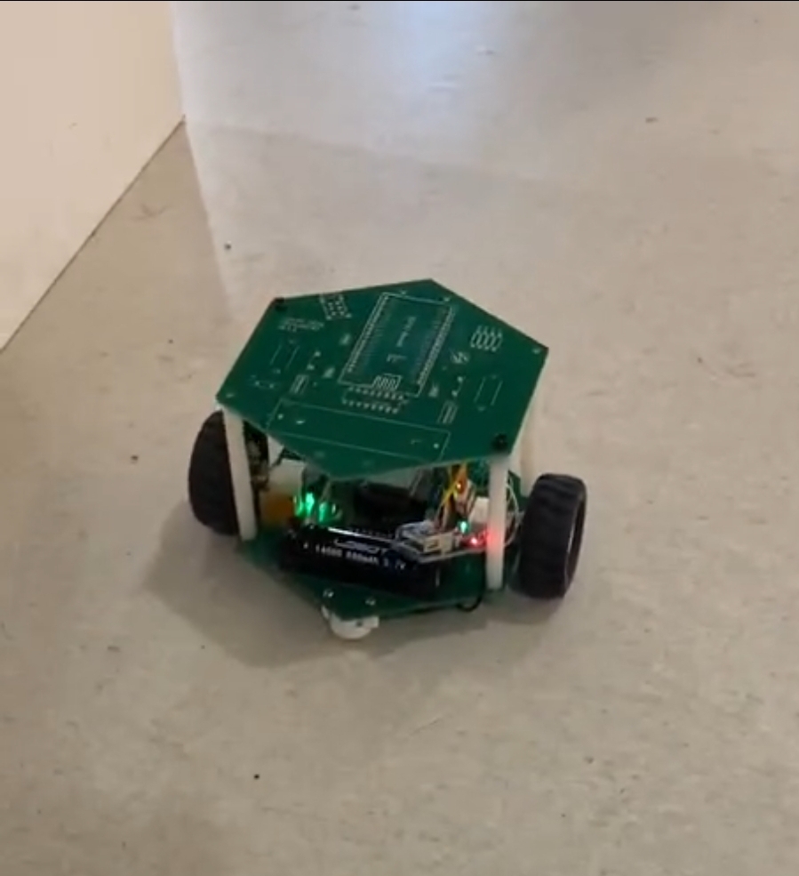
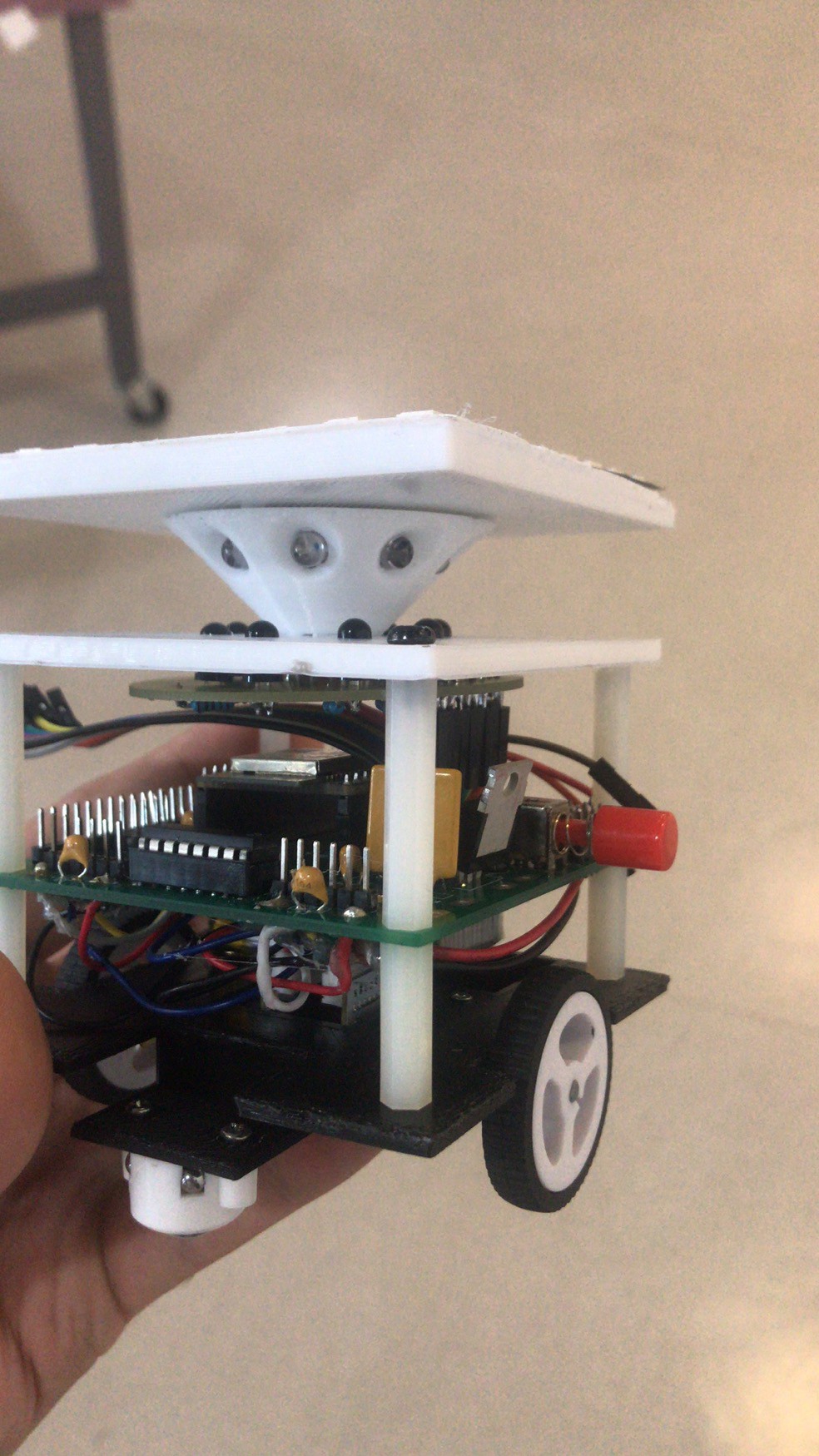
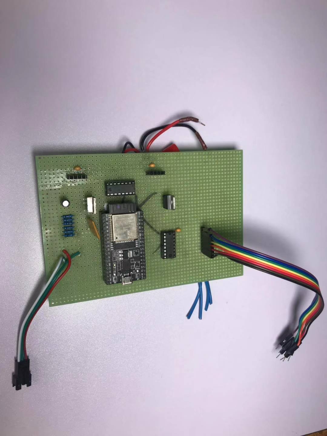
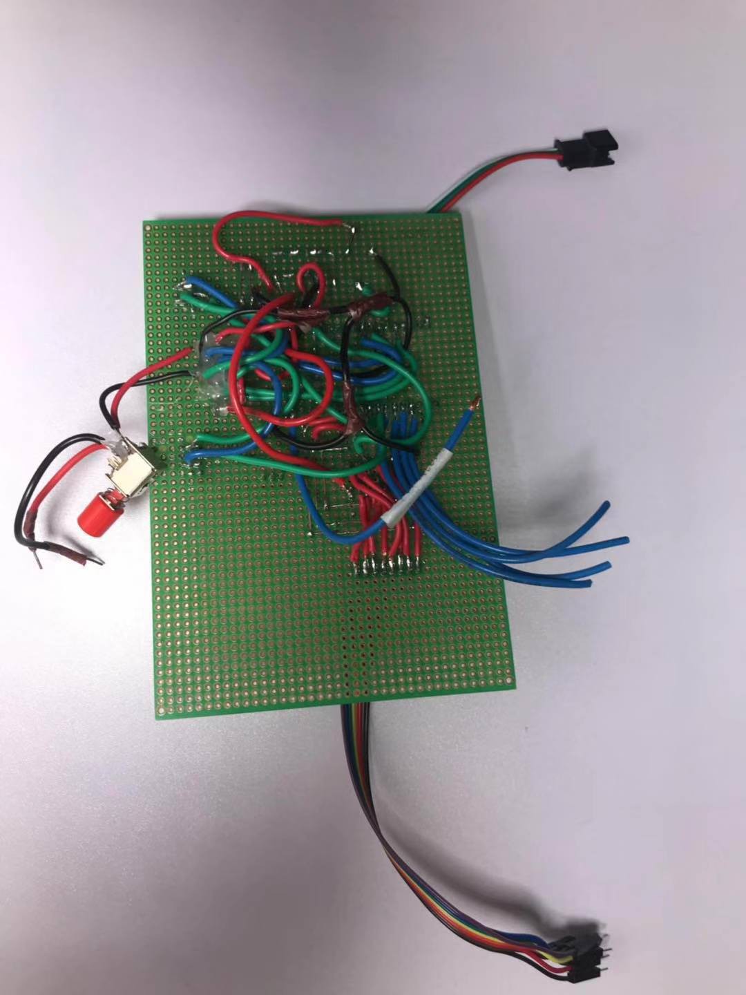
Figure 6 is an image of the assembled v1.0.2 robot. As you can see, the infrared pairs were in an awkward position on the robot. We had placed holes in the PCB for some separators between the sensors, but it was a hassle. Hence, we spent the next week testing infrared sensors and corresponding resistor values. Due to the trouble that came with the custom separators, we decided to use infrared sensors with dividers already attached to the infrared emitter and receiver pairs. As such, we used ST188 sensors, but (take note) they are not the original sizes; instead, they were 8.7mmx5.9mm, slightly smaller than the official ones.
Figure 6. Assembled v1.0.2 Robot
The resistor values for the infrared emitters were a headache for us. The 10k ohms for the infrared receivers were fine, and we didn’t change them. We set up our apparatus on a breadboard with the esp32 dev kit, five ST188 infrared sensors, and a TIP122. After changing in resistors with varying resistances, we agreed on using the 10-ohm resistors for the emitters as the proximity for detection was huge (this was the decision that caused a big problem for us later).
Before submitting our design (v1.0.3) to the manufacturer, we added an infrared emitter on the back of the robot (LTE-302) in hopes of helping other robots know when there is a robot in front of them. This addition became another one of our mistakes as we were too hasty when adding this on.
Lastly, we added three GPIO pins with +5V and GND in order for the possible addition of servos or LED matrices. We ordered five of PCB v1.0.3 for testing.
Before moving onto the discussion of the next version, there are some status updates on the wireless charging system. There was some confusion surrounding whether the wireless charging receiver can directly charge a battery, and after talking with the manufacturers, it turned out that they cannot. We were recommended to use a TP4056 module, which is a 3.7V battery charger. We had to have a battery management system to use with the wireless charging system. Since we had a TP4056 module on hand, we soldered the cables, and consequently, the wireless charging system worked great. The problem where the charging light kept flashing after two or so hours of charging was fixed. However, this also was a letdown for us to find out so late since this addition would mean the addition of two cables. Our aim from the beginning was to minimize the number of wires.
Figure 7. Schematic for PCB v1.0.3
Figure 8. PCB Layout for v1.0.3
As previously mentioned, the resistor values for the infrared sensors were not very friendly. Once we assembled the robot and programmed the infrared emitters to pulse in short time intervals, the infrared sensors ended up not working. Two issues caused this problem. The first was that the resistances were too small. This mistake resulted in the breakage of the emitters from the inside as the emitters couldn’t handle the big current. We measured a current that was as high as 1A even though the forward current of ST188 is only 500mA. After we realized this issue, we recalculated an appropriate resistance using the datasheets. Since we already had 100-ohm SMD resistors, we decided to be safe and use these. Even though they didn’t have a detection proximity as far as the 10ohm resistors, they still had a proximity of 30cm, which was adequate.
The second mistake was that although we wrote 47kR and 10kR for the resistors for the battery level pin, we missed the k when finding the correct resistors to solder onto the board.
One of these mistakes caused the boost converter to malfunction, and instead of boosting the 3.7V to 5V, we witnessed a voltage drop instead. Fortunately, after we fixed these issues, we had a working robot and were ready to make final adjustments and fine-tune the SMD pads for our final design v1.0.4.
We’ve also removed the infrared emitter on the back of the robot as we didn’t thoroughly test this emitter, and we were worried this would cause further problems. There were also some difficulties and complexities in using this in software-related developments.
A small perk of using bronze standoffs was that they could conduct electricity, and as a result, we extended the touchpads to the standoffs, designed plated holes, and these touchpads became touch poles.
Figure 9. Schematic for v1.0.4
Figure 10. PCB Layout for v1.0.4
We ordered 25 sets of v1.0.4, and asked for some help on assembling the robots. The robots came out nice and cute (controversial on the cute part). Figure 11 is an image taken during the assembly process.
Figure 11. Assembly of the robots
We had to place AruCo markers on our robots, and during the hardware developments, we had been testing the paper-printed markers on the previous 2019 model of the robots. We had to transfer the markers to our new robots, and for the robots to have a pleasing appearance, we came up with an idea to laser cut the AruCo markers. We laser cut one, tested it under the camera, and found out that at times, it was actually more stable than the paper AruCo markers. However, it also depended on the size of the AruCo marker and the size of the border surrounding the marker. We tested several with varying combinations of sizes. The size in figure 12 came out to have around the same detection consistency as what the paper AruCo markers had. As a result, we continued with this idea, and laser cut 20 sets, as shown in figure 12.
Figure 12. Laser Cut AruCo Markers
Figure 13. Robot v1.0.4 with Aurco Marker
As a backup, we also laser-cut transparent acrylic hexagons in the case we wanted to return to the paper AruCo markers. We screwed the AruCo markers onto our robots, as shown in figure 13.
After using the robots for a while, we could see further improvements to be made in maybe another version. There are two significant points.
Wireless charging system
There was a limited time for us to complete our allotted work, and as such, we had to forgo the addition of the wireless charging system, at least for this round. We are at a stage where we can add the wireless charging system if we wanted to since they are tested and ready to go. However, it would be better if we could incorporate the TP4056 into our PCB, which would make the robot look much neater in appearance.
Programmer and switch
There is a problem when uploading code onto the robot while the robot is switched on. It would break the esp32 and cause it to be no longer usable unless we replace certain components. Although we are not 100% sure about where the issue is, we hypothesize that it could be the combination of the 3.7V from the battery and the 5V from the USB that breaks the 3.3V LDO, which has a maximum input voltage of 6V. In another version, we should add a diode or another system to prevent this issue from happening. As of now, the robot works if we remember to switch the robot off while uploading code to it.
The past week was mostly for doing housekeeping with the work done in the past weeks and to look ahead, think about what to do with the platform we have so far.
Hardware:
Following the pattern of week 2, we received PCB v1.0.1 on Monday and assembled our model immediately for testing. We kept our fingers crossed, hoping that everything (or at least most) will work. Having said that, we encountered a number of setbacks as usual.
Figure 1: PCB v1.0.1
Figure 2: Robot v1.0.1
The FT232RL FTDI USB to Serial Converter Adapter was not able to successfully program the ESP32 module. After several tests and probing, we figured out the mistake was an easy fix but pretty foolish: one of the S8050 transistors was misconnected.
The RT232RL FTDI has 6 pins: DTR, RX, TX, VCC, CTS, and GND. The documentation for the ESP32 devkit asks for RTS instead of CTS, so we had to solder a cable from RTS and insert the RTS pin instead of the CTS pin for the programmer.
During the tests, we also found out that we should never use the 3.3V output of the FTDI as a power source for ESP32. It is very underpowered, as we have confirmed with a multimeter.
These three revisions then allowed for a successful connection between the programmer and the ESP32, and programs could upload without any issues.
We kept resetting the ESP32 manually by touching the ends of a cable on the appropriate pins. To avoid such inconvenience, in the next version, we will also add a reset button.
We conducted tests for each component on the PCB individually to check their functionality, and they were all successful, except for the IMU, which we are only inserting 4 out of the 8 pins, VCC GND SCL SDA in the pins for I2C. Surely, it must be another small mistake, but we cannot upload the program onto the ESP32 with the IMU inserted as of now.
We commenced the process of creating our next version PCB v1.0.2. Other than the aforementioned changes, we will also be switching the connectors for sensors modules to holes for actual sensor components (TCRT5000L, IR EMITTERS, IR RECEIVERS).
In between refining the details of component placement, we did some exhaustive tests on the functionalities that have high consumption on 3.3V. We turned on the WIFI functionality, moved the motors, flashed the LEDs, and inserted the IR modules. With these all working simultaneously, we ran the robot until it was out of juice and recharged it for a specific amount of time and measured the run time. We repeated this cycle for only 3 cycles as of now with the results as follows:
10 min charging, 20 min running
60 min charging, 100 min running
60 min charging, 105 min running
We will conduct more tests of this sort, but the pattern seems to be that the run time is twice as charging time with some fluctuations when charging time increases (to be confirmed).
Next week, we will finalize PCB v.1.0.2, hopefully, we will be able to integrate the software we have written with the hardware by the end of the week.
Software:
Last week, we tried cleaning up the software by modularizing the code, parsing all essential parts using Object Oriented Programming.
We arranged the robot’s code in the same fashion as its functionalities, divided them into classes of Locomotion, Communication, Tasks. Each of these classes has public functions exposed as interfaces. Details of these interfaces are written in their corresponding header files. In addition to these fundamental functions, we also defined another class, Robot, which holds essential properties of the robots, such as ID, current position, battery level, etc. It also integrates all the instances of the classes mentioned above, exposes interfaces that are easy to understand.
We also used a simulation software named Webots to simulate our project. With the help of Webots, we created a rectangular testing area that has the same size as our physical testing area, which is about 3 meters in width and 2.3 meters in height. Considering the workload and the shape of our robots (hexagon) that are not easy to be simulated, in this first stage, we didn’t create exactly the same robot on Webots. We only controlled its size and wheels(for locomotion) to be similar to our physical robots.
Among all the stuff involved in simulation, the implementation and adaptation of our algorithms is the most tricky one. There are lots of differences between our real implementations and the available functionalities on Webots. For instance, in our real implementation, we wrote a program to create a server using a computer network to send essential information to all the robots, such as their world coordinates, direction, destinations, and etc. Since we can’t create such a server on Webots, we use a Supervisor with an Emitter (included in Webots) instead to send the relative information to the robots. Also considering the information itself, JSON libraries are not available in Webots, which we have used in the real implementation for the sake of easy abstraction and manipulation of the information. For this problem, we currently used a string containing information in our standard format to achieve such “easy abstraction and manipulation of the information”. Besides, since we don’t have aruco code in Webots, we can not tell the robots therefore world coordinates. Therefore, we added a GPS component(included in Webots) to the robots to ensure their acknowledgement of their world coordinates consistently. We couldn’t tell their direction either, so we added a Compass component(included in Webots) to the robots. We spent much time dealing with the value obtained from Compass because certain translations are needed based on different standard directions that are set for the Compass. By doing so, we also had to change our action protocol for our robots accordingly.
After we completed our simulation, we ran it several times. It turns out that ignoring the collision, the testing results of the simulation are promising and are really similar to our real testing. In the next step, we plan to greatly reduce the errors of the moving distance and direction of the robots since we want the simulation to be run in an ideal condition that minimizes all the errors concerned. We also plan to better simulate our robots physically in its size, appearance, and its functionalities (especially components).
What’s next?
In the past week, we have been thinking about the next step. Indeed, it would be cool if we could develop our own path finding, collision avoidance algorithms and implement it on our robots. Yet as a group of undergraduate students, with limited time, resources and knowledge, this is rather hard to achieve. Here we tried changing our perspective, thinking about what we can contribute to academia, specifically within the scope of swarm robotics. Below is our conclusion after some discussion we had.
Focusing on the field of Human-Robot Interaction, implement applications such as patrolling, rescuing on our robots.
Using it as a testing platform by implementing algorithms developed by others, compare real-world data with simulation data, therefore validate their algorithm.
We received our first PCB prototype on Monday (let’s call it v0.1.0 for Swarmesh 2020)! We assembled the PCB and immediately we could see that there were several improvements to be made for the next version.
The first of which is the addition of a boost converter DC/DC for the motors, stepping up the 3.7V to 5V. This would provide more power to the motors since the motor driver consumes some current.
Another issue was the pull-up resistors near the motor driver which caused a huge problem where the robot wouldn’t power on with solely battery power. Fortunately, that was solved by replacing them with pull-down resistors.
We also need wheel cutouts on the new PCB because the sides of the wheels are touching the PCB.
Other than these issues, the test board works well and the 3.7V battery is enough to power the robot (assuming the battery has a decent amount of juice). As for the wireless charging, the ones we had were not in the best condition and we bought new ones to test. These new ones charged a 3.7V battery from 2.7V to 4.2V in 5 mins which is very fast and might even be too fast. The wireless charging system we are planning to pursue is still under ongoing tests.
Figure 1a.
Figure 1b.
On Tuesday, we started planning and structuring our new PCB (v.1.0.1). Changes and additions are as follows:
4. ESP32 documentation recommends an output current of 500mA or more when using a single power supply. The MCP1700 LDO mentioned in the last post has an output current of up to 250mA while consuming only 1.6uA of quiescent current, a far lower current than the recommended output current for ESP32. When we employ the Wi-Fi networking functionality on ESP32, it will possibly trigger a brownout or other crashes. To be able to provide at least 500mA peak power for ESP32, we compared different LDOs and eventually settled on the AP2112K-3.3V LDO which has a maximum dropout voltage of 400mV, an output current of 600mA, and a quiescent current of 55uA.
Figure 2. LDO Table
5. We shrunk the size of the PCB to a hexagon with 50mm sides. Accompanying the change to a smaller PCB, we also changed the resistors and capacitors to SMDs. The switch will also be more compact in size. The standoffs are now M2.
6.We decided to remove the devkit and replace it with only the esp32-wroom-32d module and 6 pins for the programmer.
7. Pins for I2C were added which means we can also add an IMU to the robot.
8. Two touch pad sensors
9. Analog pin for battery level
10. Three leds: one for power level, one for charging, one for state of the robot
11. Two sets of pins for two reflective sensors
12. Five sets of pins in the front of the robot for 5 pairs of IR sensors. We used to have a mux to increase the number of analog inputs, but since we have enough analog (ADC1) pins on the ESP32, we refrained from adding a mux to save space.
In the following week, we will be receiving PCB v1.0.1 and assembling it. Hopefully, everything will work as intended.
Figure 3. Schematic for v.1.0.1Figure 4. PCB layout for v.1.0.1
Software
This past week has witnessed enormous software progress we made. Based on the camera system and tests implemented last week, we now can give the swarm of robots a list of destinations to go to, the robots would then figure out the destination they should go to.
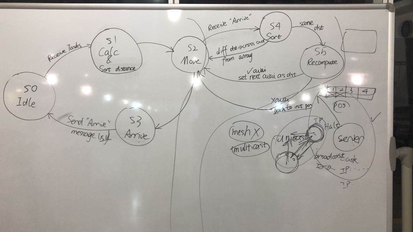
The logic of the system follows the Finite State Machine shown in the last blog post. Robots would receive the absolute position of all robots as well as positions to go to in Json documents delivered by multicast. Each robot would pick the destination with the least Manhattan distance with regard to its current position. When a robot arrives at its destination, it would again send a multicast message specifying certain coordinates are taken. For other robots which also picked the same destination, they would pick the destination with the least Manhattan distance from the list advertised by the server. For robots that didn’t pick the same destination and have not yet arrived at their destination, they would delete the destination from their lists. If there are more robots in the system than the assigned destinations, robots that don’t have a destination to go to would go back to the spot before any task was assigned.
Same as the grid system in Manhattan distance, the robots always go in a straight line, turn 90 or 180 degrees when it needs to.
The above functionality was achieved with the code we wrote this week. Of course there are still potential bugs in the system; it would usually take a lot of time for the robots to go to their destinations. But in general, the system works.
In the coming week, we will work on
1. PID algorithm for the robots, so that the robot wouldn’t suffer from undershooting or overshooting when turning and moving forward.
2. Draft collision avoidance protocol, which we will discuss in other parts of the blog.
3. Put the collision avoidance protocol into the simulation platform.
We also did some literature review on collision detection and avoidance. We found two articles that are really similar to our project, which are “Multi-sensor based collision avoidance algorithm for mobile robot” and “Collision avoidance among multiple autonomous mobile robots using LOCISS (locally communicable infrared sensory system)”. Both of them, in the first place, gave us insights on which sensor(s) may be effective for us to apply to our own robots. Considering many other articles, sensors like cameras, IRs, ultrasonic, and etc. are commonly used in such a system. Furthermore, we get to understand the protocols of collison detection and avoidance for both static and dynamic obstacles better. It may be helpful for us to develop our own protocols for our robots in our testing area.
Attached are demo videos of the robots moving and assigning tasks
It's been half a year since we last updated the entry. Recently we talked again about our direction and progress. We realized to make Swarmesh a candidate for distributed system research, we first need to develop a platform with all functionalities integrated and readily available
Necessary improvements to be made on the system are listed below.
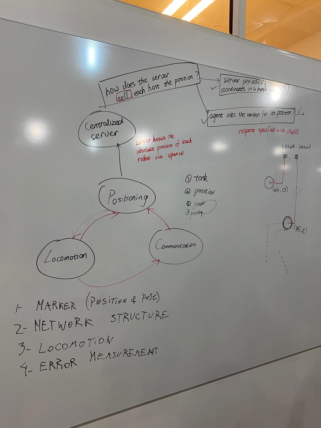
1. Positioning system
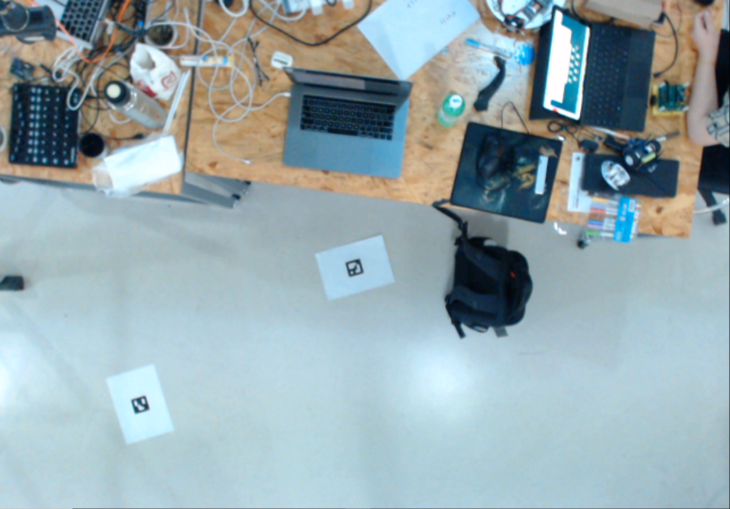
Though last year we spent a lot of time & effort on the distributed positioning system using IR, the petal shape IR radiation and the limited detection range were really bothersome. In this iteration, we decided to give up on the IR positioning and turn to having a camera hanging on the ceiling pointing down at the floor. To recognize the robot, each robot carries a unique arUco code on its back. A computer connected to the camera would use OpenCV to analyze the image and output the coordinates of all robots in the image. These coordinates would then be multicasted to an IP address using UDP. The UDP packets would be sent periodically, to guarantee the robots don't go off-course.
2. Communication:
As mentioned above, we are using multicast for terminal-robot communication. The robots would be subscribed to a multicast IP that's dedicated for providing position information. We used mesh for robot-robot communication in the past, yet the tests we ran last year showed the communciation is always unstable and has a very limited range. There is also a chance that we get rid of mesh and turn fully to multicasting. But at this point we have not decided yet.
3. System structure
We are envisioning the system to carry out tasks like shape formation. The robots would receive tasks from the centralized server for coordinates to be taken up with. Based on Manhattan distance, the robots would distributedly calculate the nearest destination. They would move to the destination according to the Manhattan distance calculated.
Plans
The steps to develop the system are shown in the pictures below with order.
Finite State Machine of each robot
Week 1 Progress
Mechanical
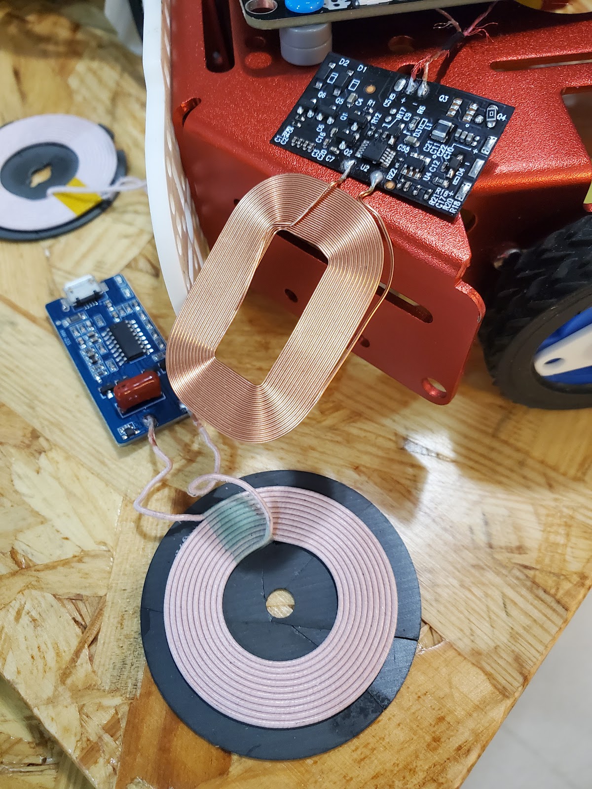
Wireless Charging:
We are experimenting with wireless charging modules and 3.7V rechargeable batteries, which is significantly easier than the wired charging with the 7.4V Li-Po battery packs on the previous design iteration. No more fiddling with cables. No wear and tear. However, some possible drawbacks include overheating and slower charging time.
Some tests with the wireless charging modules were conducted on the KittenBot (by soldering the receiver to the battery) to test the capabilities of the system. The results show a consistent pattern where the runtime is twice the charging time. However, the battery on the KittenBot is 2200mAh 3.7V, which is slightly different from the smaller 3.7V batteries (around 850mAh) that we intend to use. We predict that the smaller 14500 3.7 batteries will result in a runtime of around 4-5 hours.
Motors:
Since we changed the previous 7.4V Li-Po batteries to 3.7V Li-ion batteries, we also want to test out the 3V 105rpm gearmotors with encoders. As for improvements in cable management, we will be using the double-ended ZH1.5mm wire connectors, allowing us to easily plug and unplug motor cables from the PCB (if you recall, the wires were soldered onto the PCB in the previous version).
PCB:
We have designed a test PCB on Eagle (and sent it to a manufacturer) that can accommodate the new changes mentioned above. Another addition is an LDO Regulator (MCP1700) to regulate a 3.3V voltage for the ESP32. We are also trying out a new hexagonal shape for our robot. Let’s see if we like it. The plan is to examine the efficacy of the wireless charging system and examine whether the smaller 3.7V batteries can provide enough power to the motors and the ESP32.
Software
OpenCV
We first tried to learn open-cv to become more familiar with this new module, which is probably one of the most important and fundamental ones. After that, we proceeded with our project on the base of Zander’s code on camera calibration and arcuo code detection. We fixed bugs including how to invoke the right webcam connected to the computer and using the os module to better specify the file path, which ensures the code to be executed correctly on different machines. We also made some improvements on the aruco marker detection code. We used “adaptive thresholding” to reduce the influence from the shadow and natural light, which seems to be ruseful. We also used “perspective transformation” to make the camera better focus on the testing area, thus reducing the error of the world coordination (to around 5 cm?).
Multicast
We tested sending multicast from Python and receiving from ESP32. The terminal sending muIticast and the ESP32 receiving multicast are all connected to a LAN. The terminal emits multicast every three seconds. The tests showed very promising results. There is little delay in getting the message; the packages weren't corruputed during the tests as well, even when a large chunk of data (500 bytes) was sent.
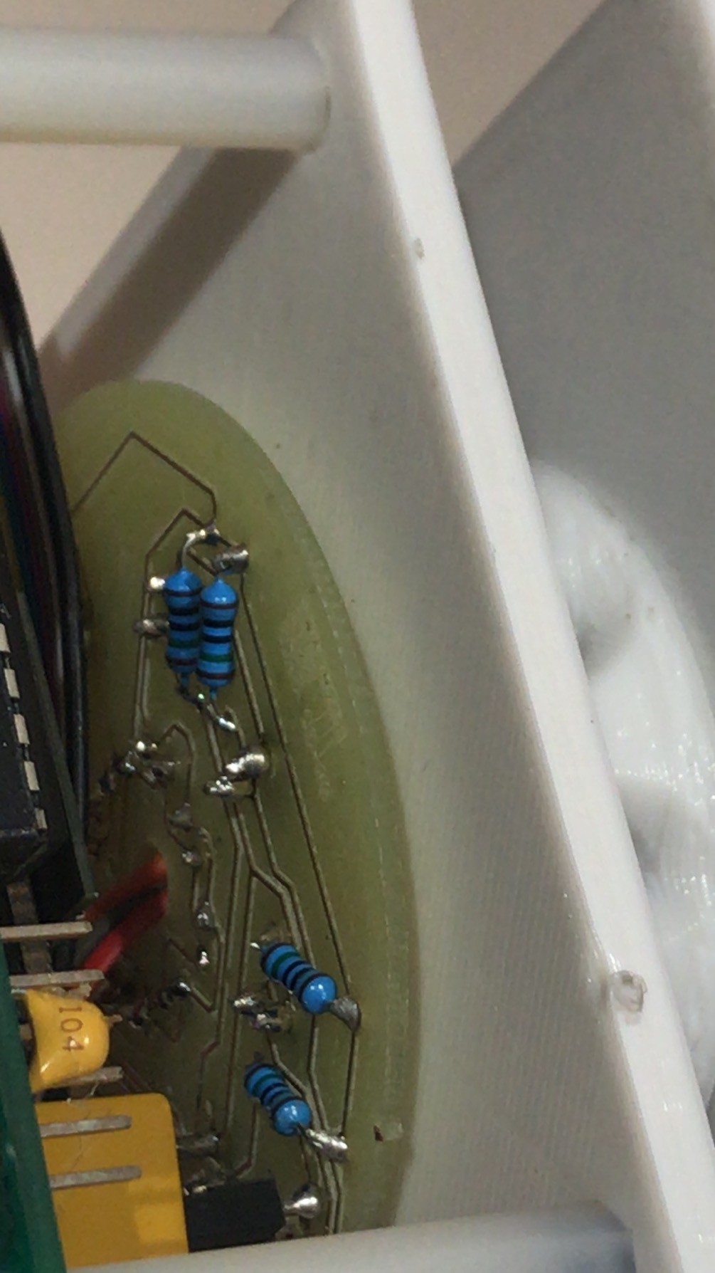
We started to assemble the infrared relative location circuits but it took us more than hours for the first two pieces. We spent other four hours to test their functions, finding many issues that were conflicting with the design. It was critical to our success that our previous test of the IR location was rigorous (with all the data shown in our research paper) and that we were able to reconfirm the working circuit re-assembling the original prototype. Our next steps move towards a redesign of the circuit to try that modified implementation.
Issue 1: Industrial design
The steps of the original design for the prototype were:
- assemble infrared(IR) receivers, connectors and resistors on the printed circuit board (PCB)
- mount 3D printed base plate
- mount 3D printed reflector cone
- insert 8 emitters (guessing the position of these 16 pins was possible took us 80% of the time)
- solder the 16 pins
- desoldering many of the pins because of guessing their position wrong. Resolder. Solder again.
Issue 2: External capacitors for ADC ultra-low noise pre-amp
Pins 3 and 4 of the ESP32-DevKitC were in our schematic expected to be used as analog read and to be connected with infrared proximity sensors, hence they had pull-up resistors. After digging about the extra functionalities they have, they have functions related to the pre-amplifier of the analog digital converter. The manufacturer suggests to connect a capacitor of 330pF between these two pins to get ultra low noise.
We didn't try that, but we can make sure we wouldn't be able to use the pull-ups and the ADC functions correctly. We noticed this when there was a mysterious grass noise on the readings (about 20% of full scale!) but as the IR were not even installed, we removed the pull-up resistors and the analog values came back to normal.
Issue 3: Circuit design
Pin 2 fo JMUX connector was noted as being Vcc on the IR board. But on the main board that pin was coming from a resistor in order to limit the current through the IR transmitters.
Also we had to resolder all receivers because they were noted as phototransistors but they were inverted diodes instead.
So far we have been switching from MicroPython, Arduino IDE, Platformio to IDF. Now that we are tuning up the first prototype, we are re-exploring the needs of our swarm network.
Espressif provides an insightful explanation about how it handles MESH communication:
So far we have been working with their IDF environment to develop basic tests. Surprisingly enough, there is an Arduino Library that could make our work approachable by beginners: painlessMesh.
With the first tests of this library, one of the essential things that we noticed was that nodes were dropping and re-appearing. Also the switching seemed to be a bit mysterious, so there was a bit of reluctance in our team of handling a black-box. So we decided to investigate MESH a bit more.
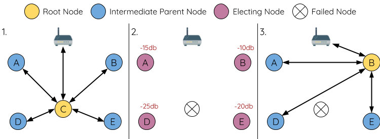
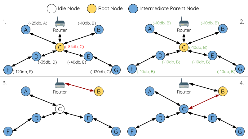
The first key concept that was key to understand the behavior was the automatic root node selection.
Another concept that helped us understand what was going on was this diagram for root node switching failure.
Among these, some of the node behaviors were clearer. Still, the painlessMesh library has many dependencies and among them, the examples use a task scheduler. This was far from ideal for our application, but thankfully we realized that MESH takes care of all the internal switching and that handling the data stream is up to the user software.
There has been a quiet period here but it was mainly because we were working on hardware issues... that were indeed hard. We will at least share that the schematic using ESP32 in a MESH network was tested and the IR location multiplexed was also a success.
The steps we are working on now are to bring to life a whole robot. In order to do this, we used Eagle to design a Schematic, later hard wired it to a perfboard and designed a PCB based on that test. After running a small test on our Protomax, we are now waiting that the factory ships the prototype boards. Let's keep fingers crossed!
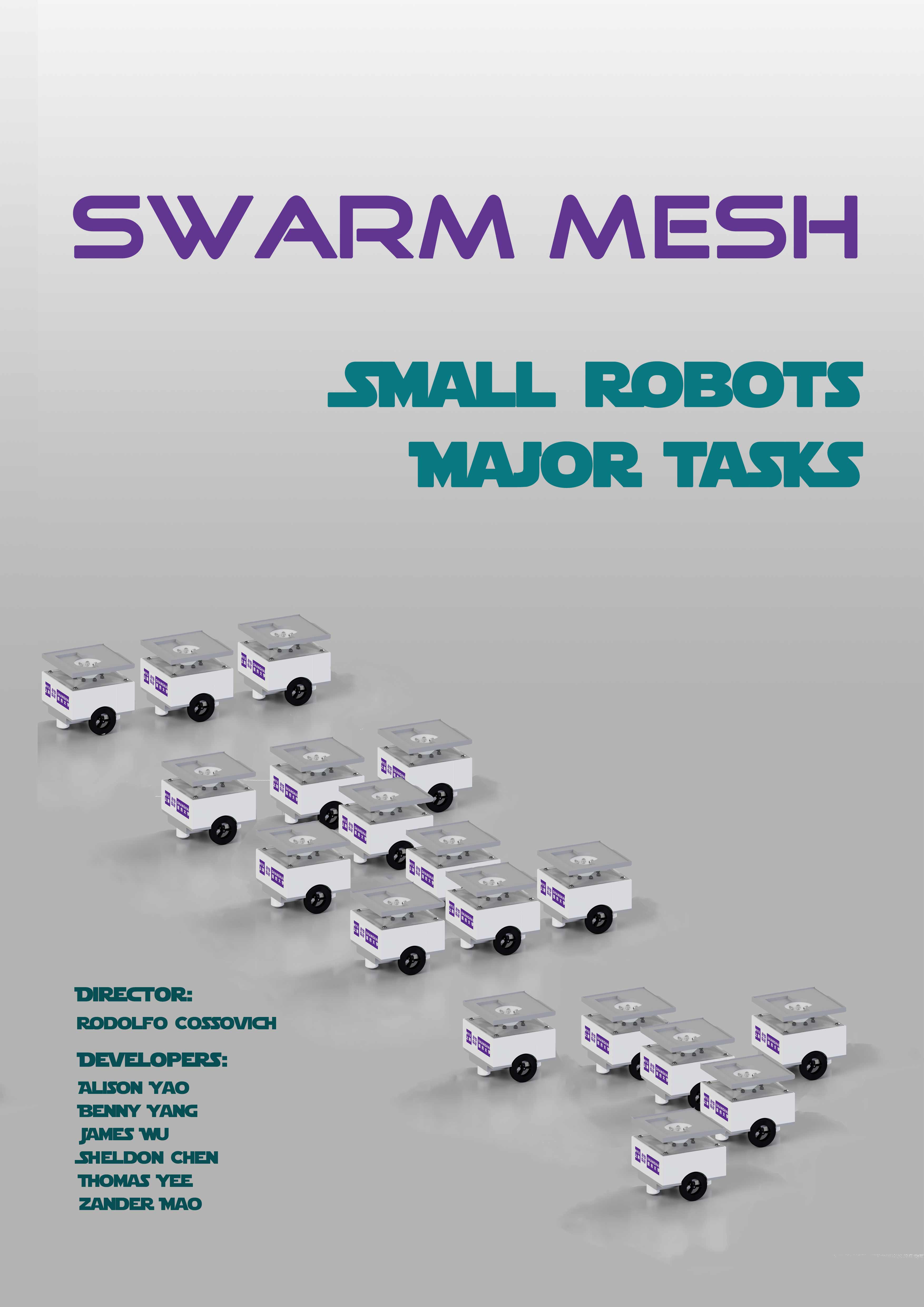
The poster features the rendered 3D model of the swarm robots, which come to form the word of IMA. This is demonstrates one of its key abilities, forming shapes or images. It can be used to achieve robotics art in future application.
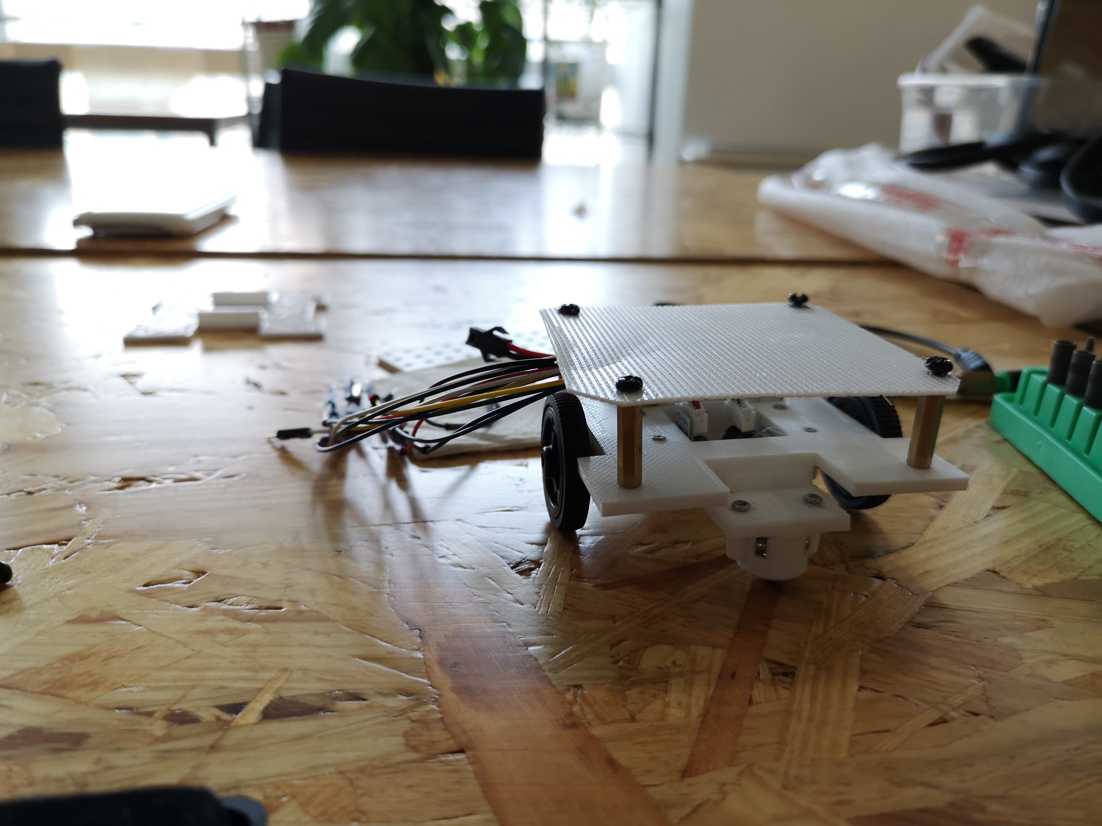
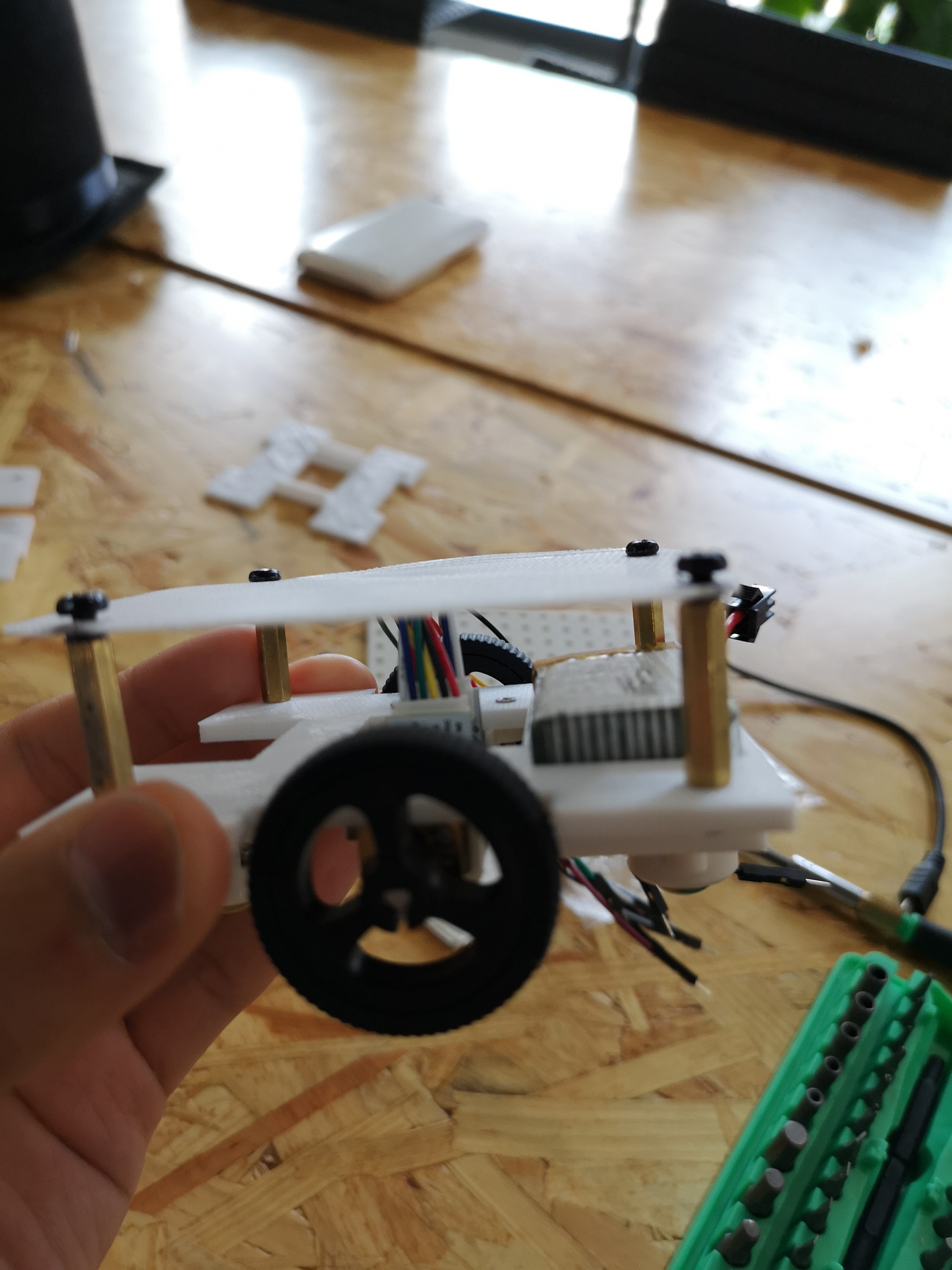
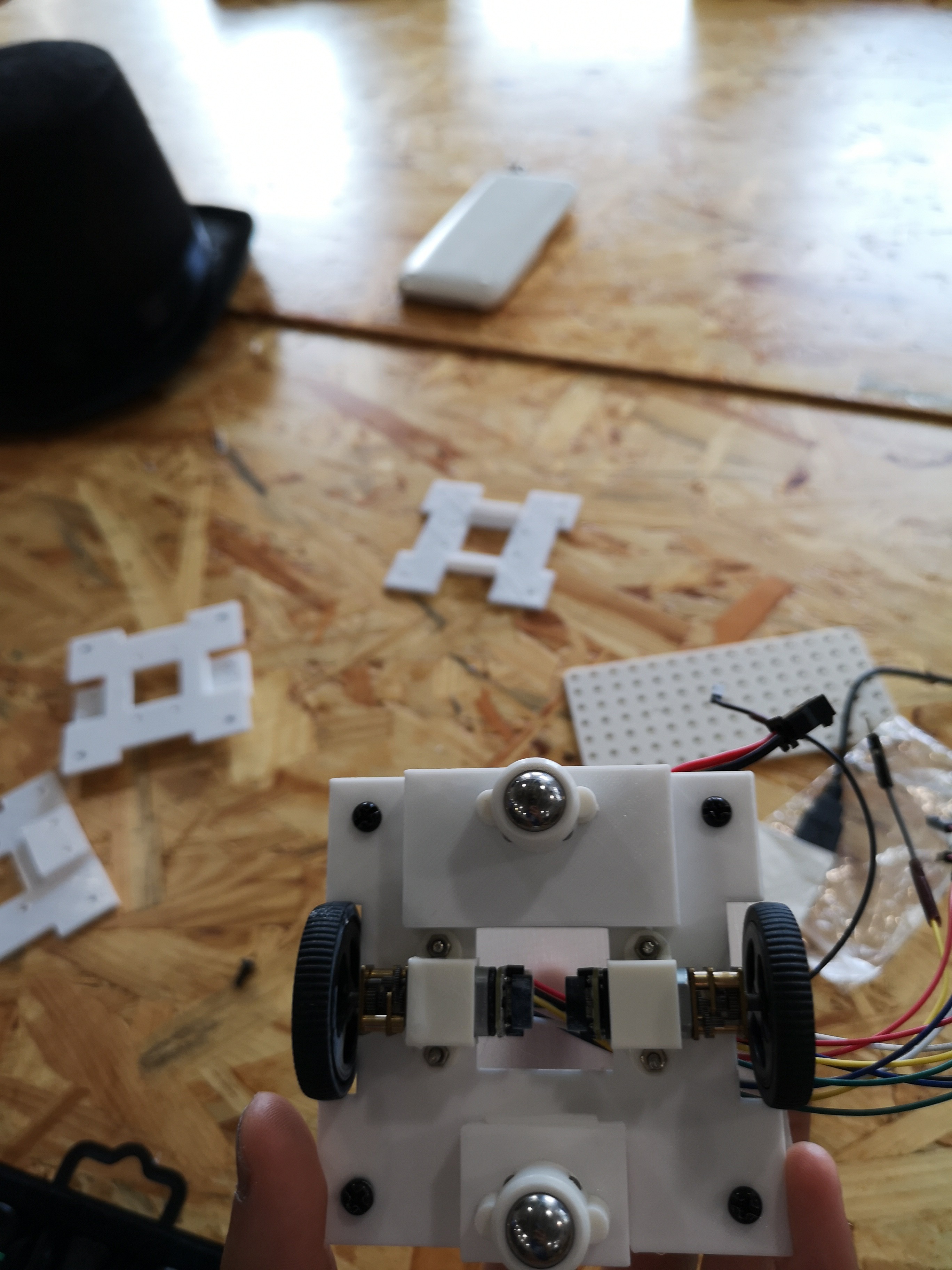
First let us show you how the chassis of our swarm robot looks like:
The four screws are used for attaching PCB with the chassis. There's a groove where the battery lies. In addition, the cables controlling the motor go through the middle of the chassis and will be attached to the PCB above.It has two wheels with motors, and two little balls attached to keep the robot balanced.
And this is the 3D model of the chassis that we built through Fusion 360
When we were building the model, we took several things into consideration.
1. The total size of the chassis cannot be over 80*80mm too much
2. Two wheels with motor on it need to be attached on it
3. There should be four holes to attach the chassis with PCB using screws
4. We'd better leave a hole in the middle of the chassis such that the cables attached to the PCB above have place to go
5. The chassis needs to hold the battery
6. Two balls should be attached on the other two sides in order to keep the robot stable.
Taking all the details into consideration and after several modifications to the prototype, we've come up with the first "most-satisfying" version, fitting all these requirements. Further progress of chassis construction will go along with the whole team's process, let us wait and see :-)
 Rodolfo
 Figure 1. FLow chart of task assignment
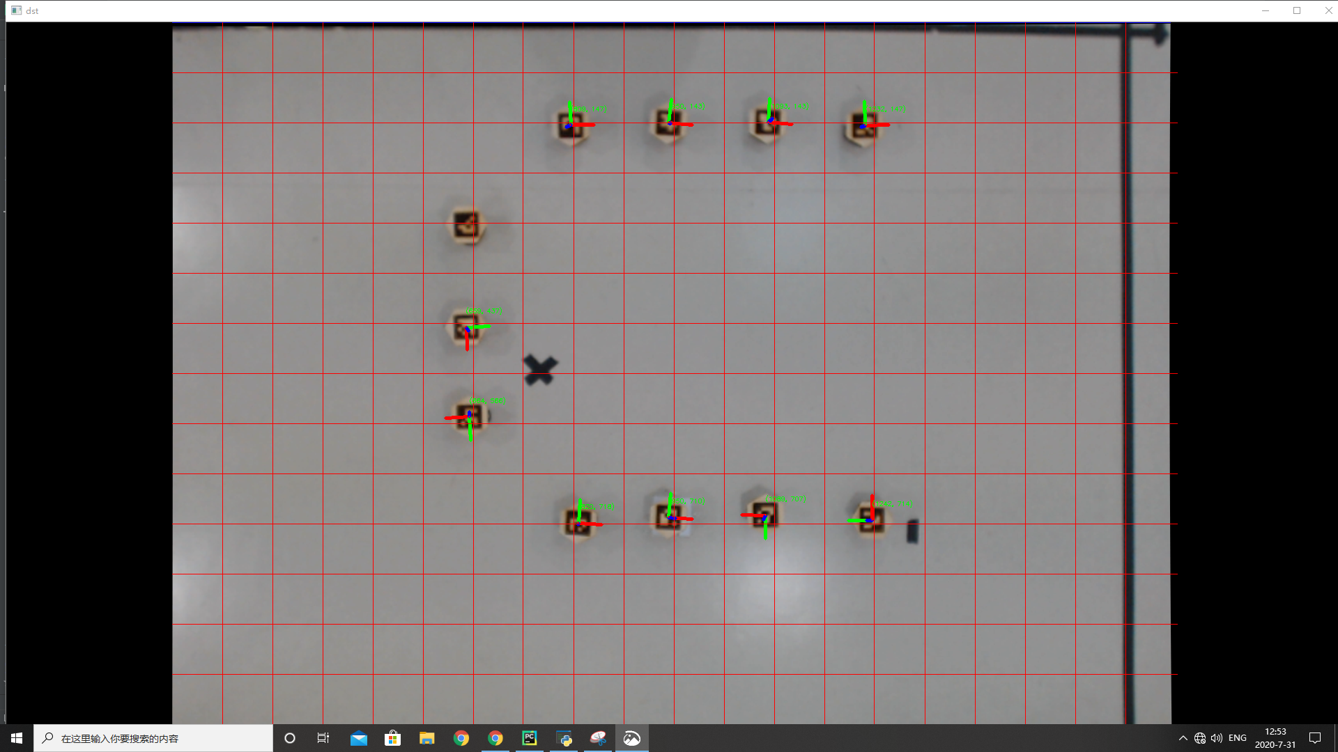


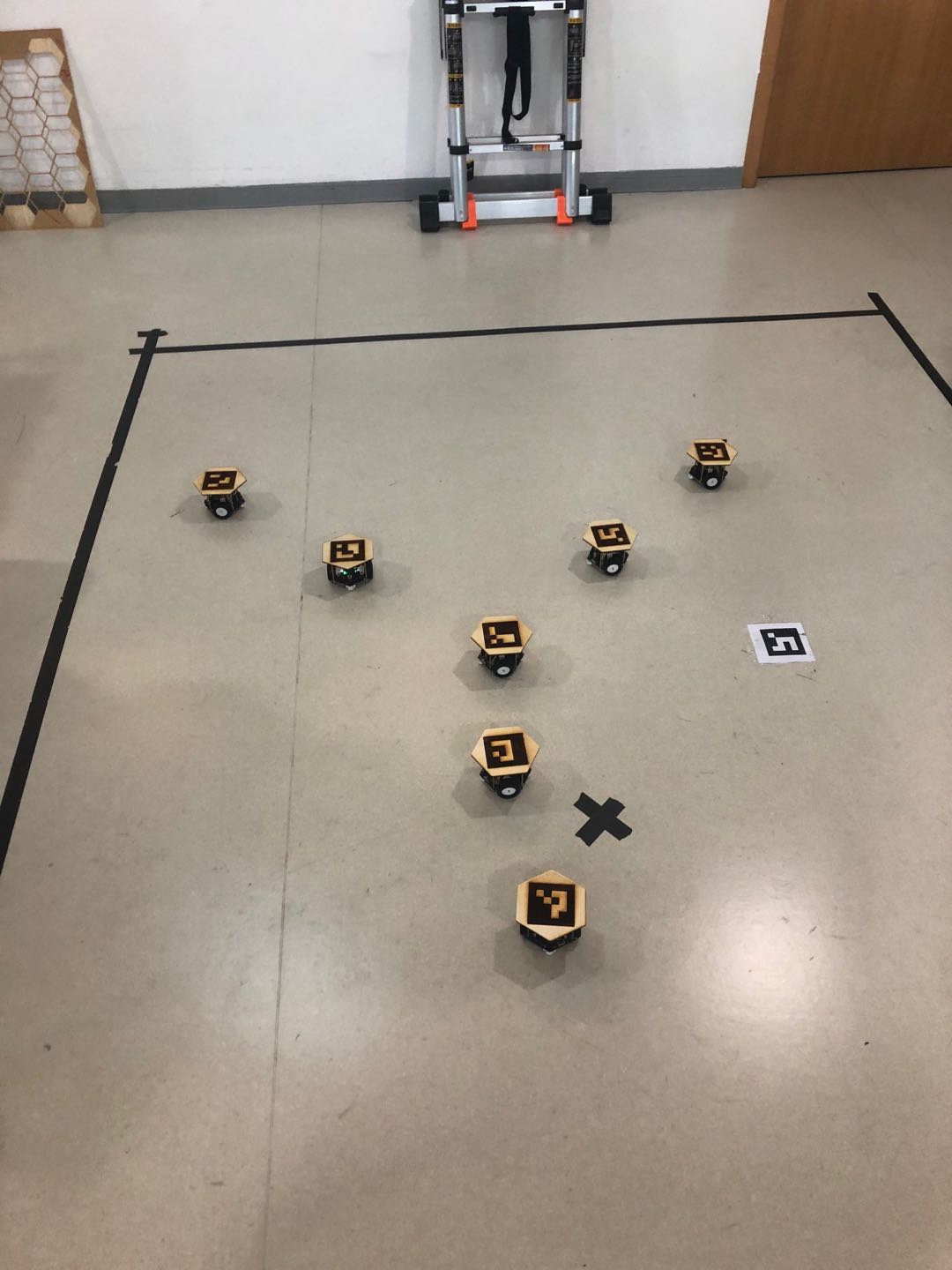

 Figure 8. “Component-based” modeling

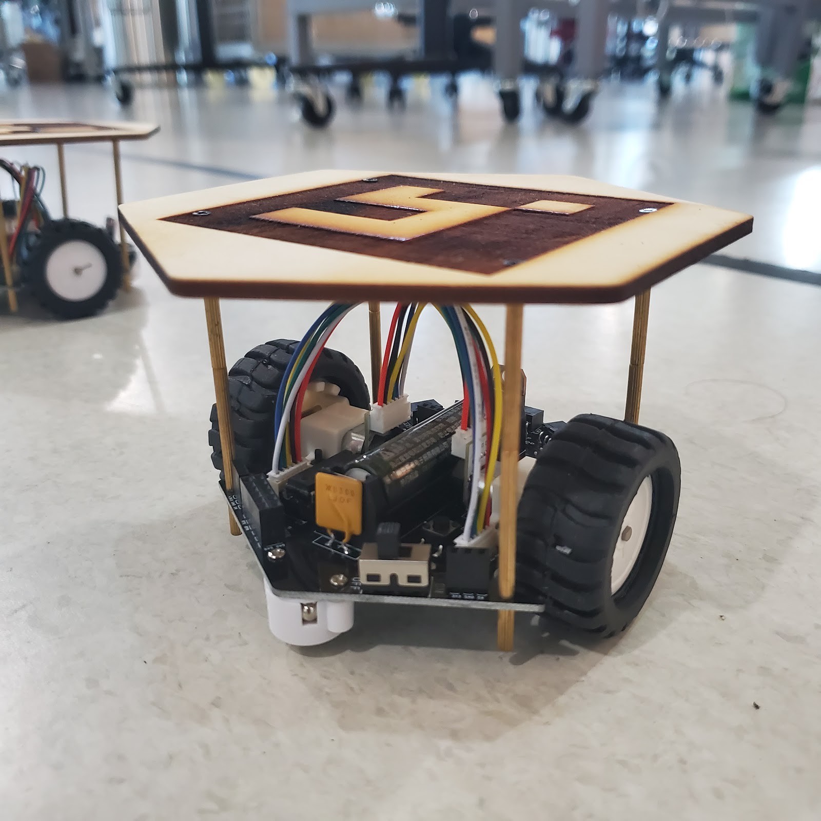


 Figure 3. Receiver plate design
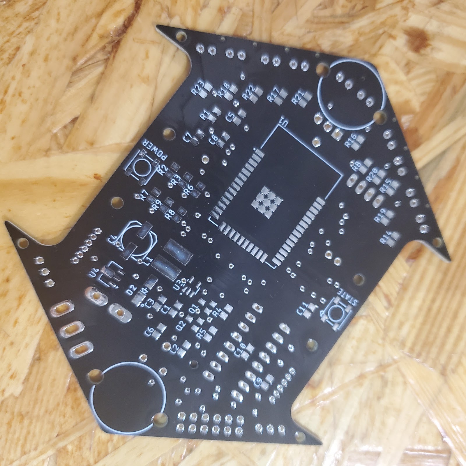 Figure 4. Bottom view of PCB v.1.0.2
 Figure 5. Ai Thinker USB TO TTL Programmer
 Figure 7. Schematic for PCB v1.0.3
 Figure 8. PCB Layout for v1.0.3
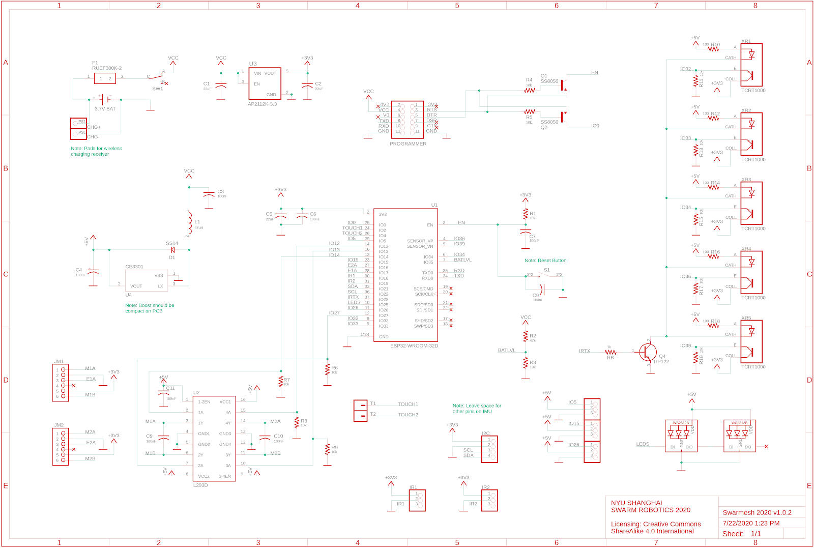 Figure 9. Schematic for v1.0.4
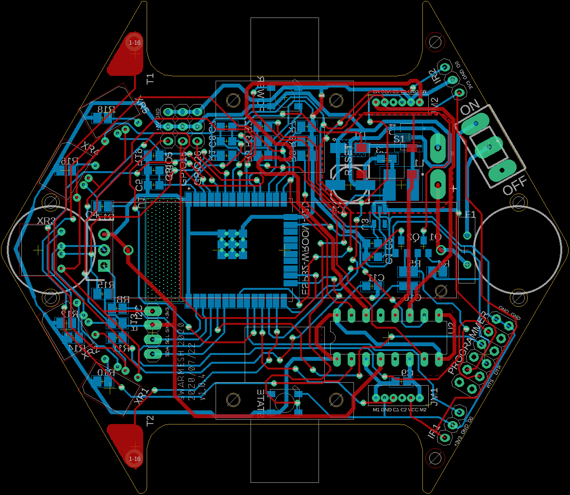 Figure 10. PCB Layout for v1.0.4


 When we were building the model, we took several things into consideration.