A second test was carried out within an urban single-unit household in Kibera informal settlement. Actual names have been altered in order to keep identities private. We thank them for offering us the opportunity and permission to collect and analyse their data and make it public for the sake of public awareness. Asante!
Meet the family :)
John Doe* has lived within Kibera for the past 16 years, he met his wife Jane Doe* within Kibera. They are married with 2 children: A girl aged 15 years in a local day high school and a 6 month bundle of Joy. They live in a single room made of aged iron sheets roughly measuring 2 meters(~12 feet) by 3 meters(~36 feet) that they share with their 2 children. They also cook within this single room. Amenities such as bathroom are shared. There is electricity but illegal connections causing fires in the neighborhood have made them afraid of connecting their home to the grid! They thus use candle for lighting. The household energy mix includes charcoal briquettes and kerosene. Kerosene is mainly used during the day while briquettes are used in the evening.
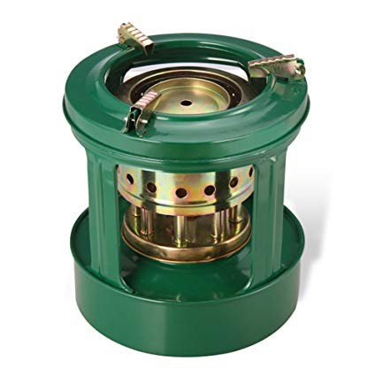
A sample kerosene stove
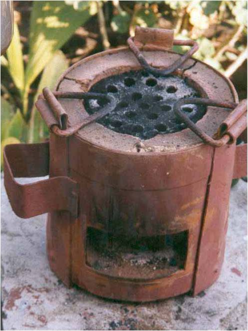
A sample briquette stove
Data analysis
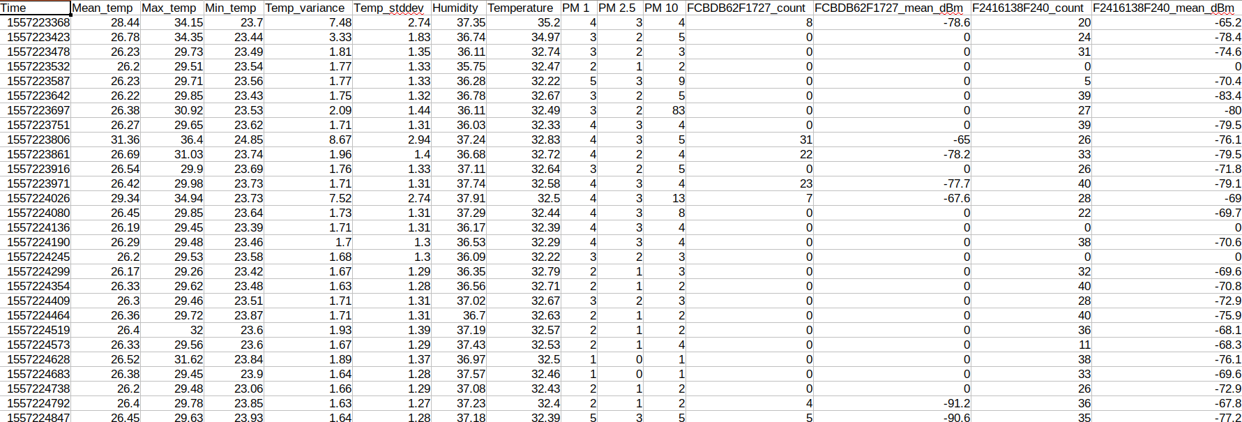
Data was captured in a CSV file as below using an OpenHAP unit and analysed.
The above image shows raw data collected.
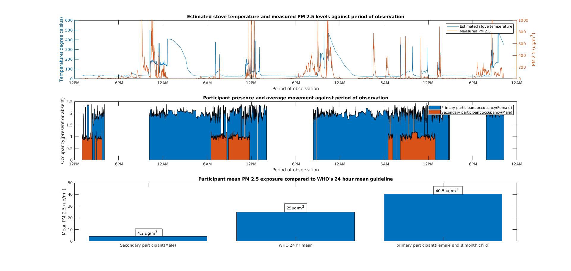
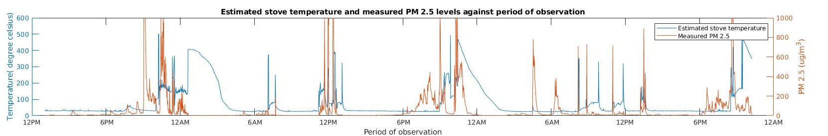
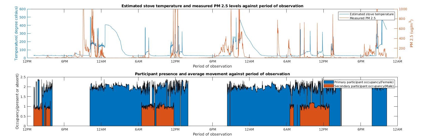
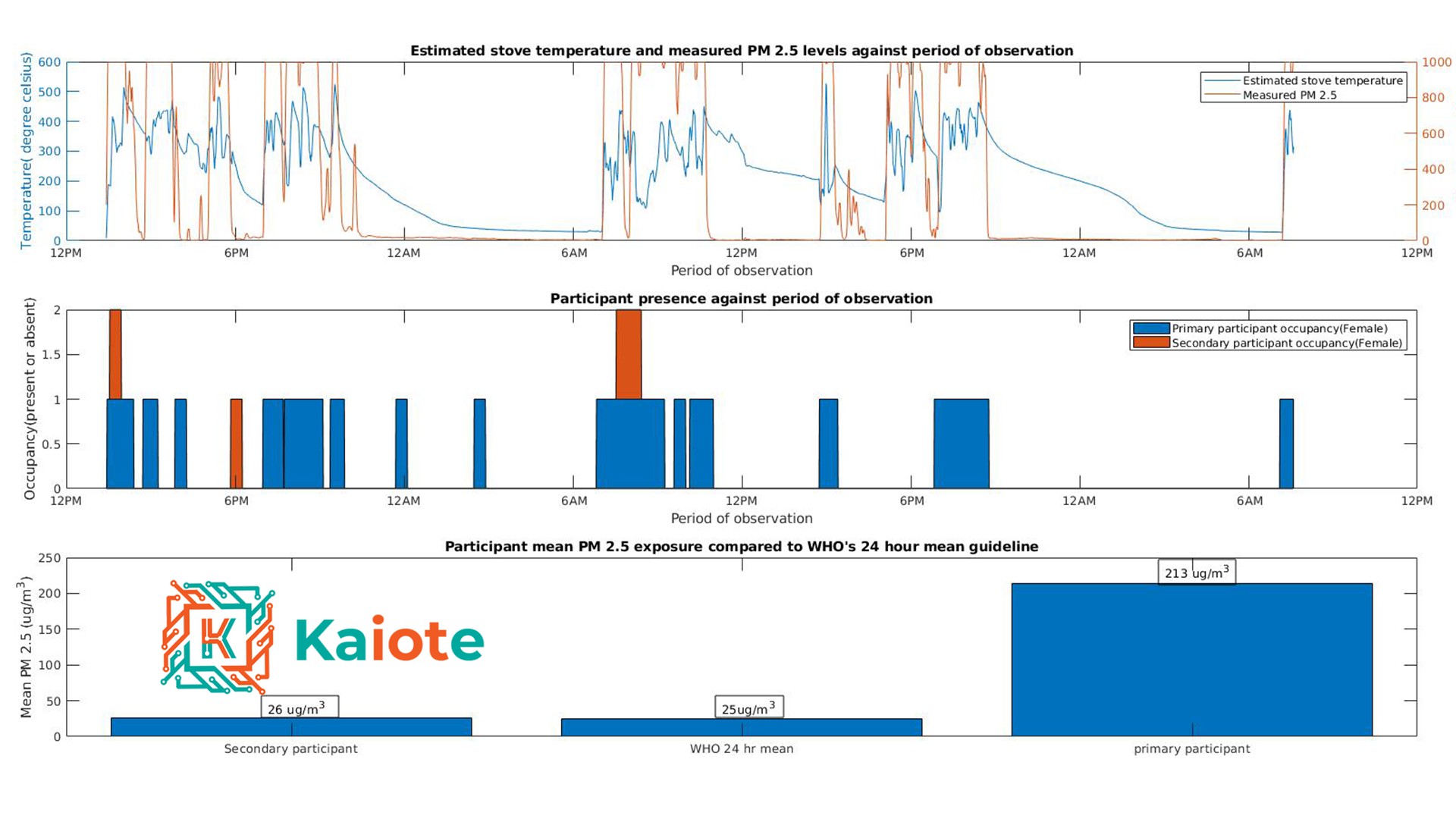
Plotting MLX90640 max temperatures, PM2.5 values against time
Tp obtain the plots above of stove temperature and PM2.5 against time, the unix time recorded in column 1 is converted into ISO 8601 format, the day , hour, minute, second is extracted and plotted on a continuous line. The corresponding values of PM2.5 and Max temperature(Obtained by pre-processing the MLX90640 pixel data before saving to the CSV file on the SD card) are plotted against this.
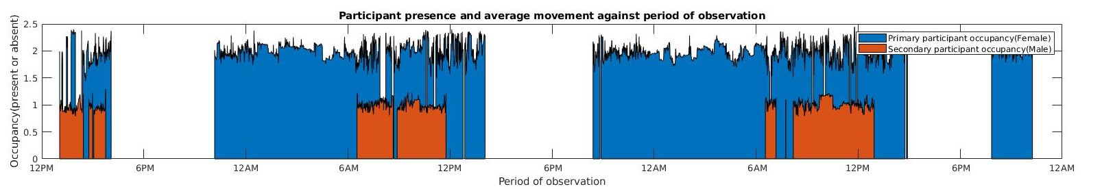
Overlaying activity information on presence information
We obtain
The above plots are a superposition of two datasets:
Presence information - Derived from "<BLE_MAC>_count" column in the CSV file. This column stores the total number of messages received in that specific data acquisition cycle from a wristband identified by its MAC address. A zero value represents absence while anything greater than zero shows presence.
Activity information - Inferred from "<BLE_MAC>_mean_dBm" column in the CSV file. This column stores the average signal strength of the total number of messages(RSSI monitoring) received in that specific data acquisition cycle. This is because a wristband typically sends messages every 1-3 seconds whereas a typical data acquisition cycle lasts 20-40 seconds depending on settings.
The Y axis can take a universe of two values with regard to presence/absence:
Y value > 0 -> present - In order not to have the same single level for various monitored persons, we settle for unique integer values per person with regard to presence. In the graph above:
Value 2 represents primary participant presence.
Value 1 represents secondary participant presence.
Y value = 0 -> Absent
As we can only measure the activity when the participant is present, we superpose activity information on the presence information. To do this we scale the dBm information and overlay in on the presence plots above.
The more variation there is, the more active the person. This can be used to infer when one may be asleep or awake.
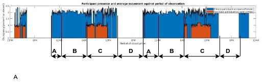
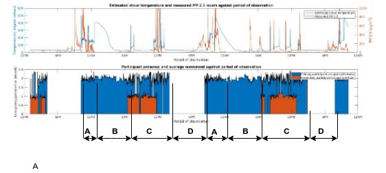
Analysing presence/activity information
The primary participant here represents an actual mother with a six month old child. She takes care of her child as is with it 24 hours a day. A typical day is split as follows from the data - You do not even need to know the household culture to see what the data is telling you:
A - She comes home at around 10 pm daily.
B - She sleeps at around midnight and wakes up at around 6am before the secondary participant - her husband comes from work- We later got to find out after data collection and analysis that he works as a security guard in an upmarket estate in the capital.
C - While she is awake, the secondary participant - her husband does some activities around the house before sleeping for around 1.5 hours and waking up again to leave at around midday.
D - She leaves the house from around 2pm till around 10 pm - We later got to find out after data collection and analysis that she runs a grocery shop that she tends to over this period.
Cycle continues.
Analyzing presence/activity information with pollution information
Before A - The pollution levels are moderately high The stove is out of thermal camera view. This was actually a data gap but after enquiring on this we are told the daughter lights up the stove and warms it before the mother(Primary participant) gets home. The reason for this is because the briquette stove takes some time to get lit.
A - She comes home at around 10 pm daily. The pollution levels peak. -After analysis, we were told that she cooks with the briquette stove as soon as she is home.
B - She sleeps at around midnight, the temperature peaks because the stove is in view of the thermal camera. The husband comes in at around 6pm, the heat from the stove has long subsided around two hours prior- We were later told that she uses the residual heat to warm the room. This presents a danger of carbon monoxide poisoning without their knowledge, putting her life and her children at risk. The husband is not present at the moment.
C - She now uses the kerosene stove to quickly cook breakfast, represented by the short temperature spike. Particulates are minimal! She then cooks again at around noon, sharp temperature and pollutant spikes are noted. - From information, this is still from the kerosene stove.
Cycle continues.
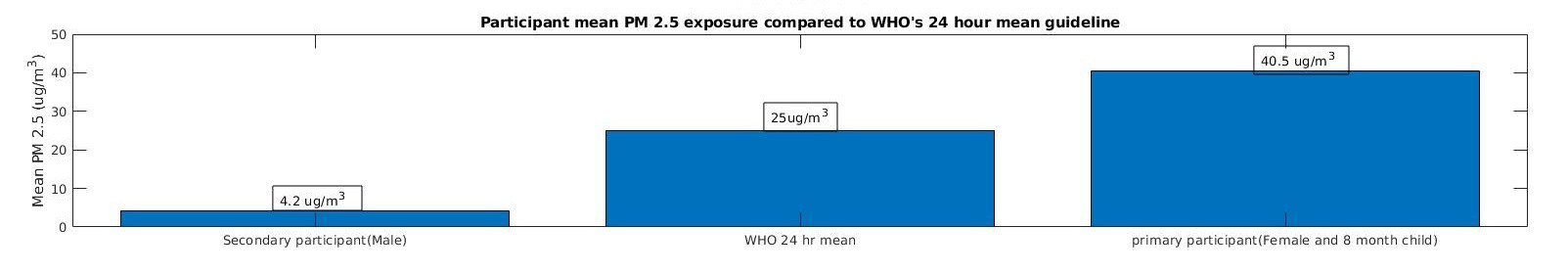
Calculating pollutant exposure
The indoor pollutant exposure is calculated by getting the mean of the pollutant levels. This is calculated as below:
When a participant is present, the pollution exposure is equal to the measured value by an OpenHAP unit.
When a participant is absent, the pollution exposure is assumed zero! We take it this way as our scope does not extend beyond the kitchen wall perimeter.
As can be seen, the husband is negligibly exposed, with his values being 5 times below the WHO limits. The wife and the 6 month child receive majority of the exposure and are around 1.5 times the recommended limit. In addition, this does not consider the carbon monoxide poisoning leading to slow suffocation! We did enquire about this but they did not know the effects of CO poisoning given they have not had the priviledge of education and I would not blame them but it is important that they now know the effects and have changed to cooking in open spaces outside!
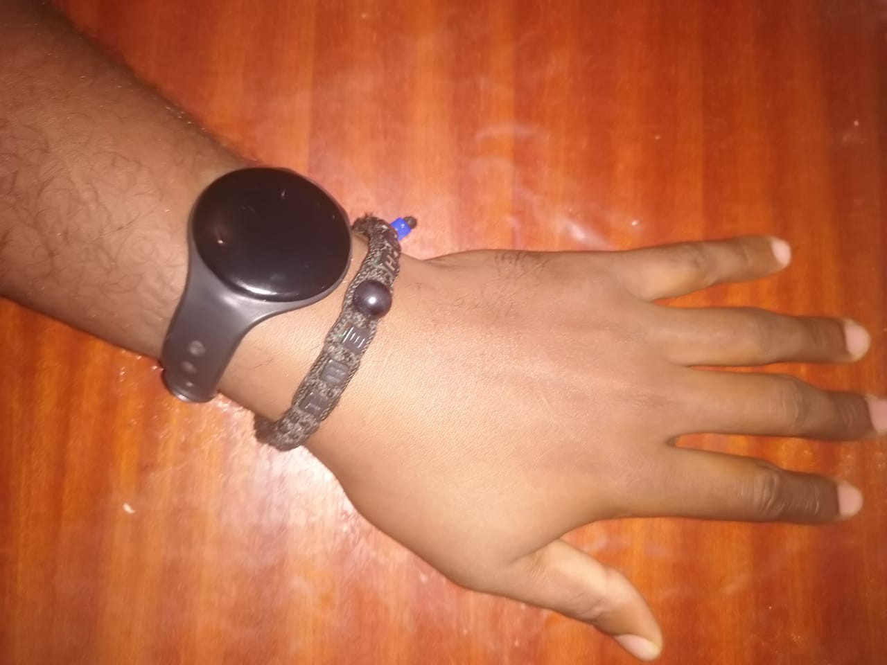
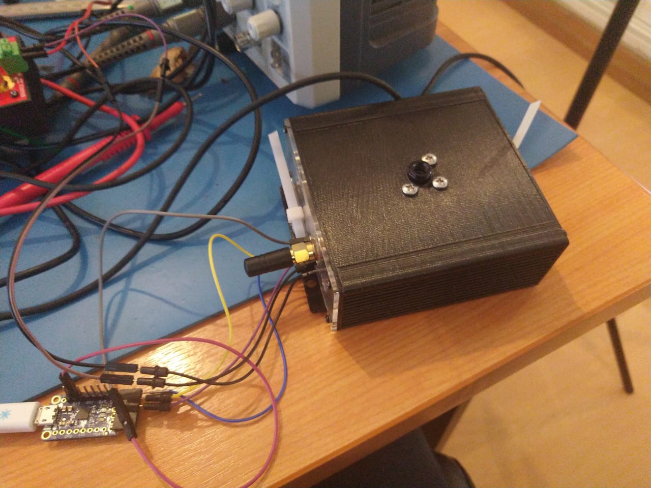
A bluetooth tag that supports Eddystone / Ibeacon BLE protocols is used. This would allow the ESP32 to monitor human behavior that may have influences on pollution.
With each Eddystone TLM(Telemetry) frame we would extract the beacon count and its associated RSSI.
Tp ensure that the beacons are not received outside of the kitchen, we reduce the output power of the radio using the manufacturer's android application till the beacons RSSI outside the area monitored are below the receiver threshold.
Configuring beacon interval and output power via manufacturer android application
For the webserver we chose the libesphttpd project, originally created by Spritetm, originally for the ESP-8266 but modified for the ESP32 by Chris Morgan.
Purpose
The purpose of the webserver is to stream data to a mobile handset or computer using the onboard Wifi ability of the ESP32. The use of the webserver was designed to be primarily used to set up the system and ensure the system is okay prior to leaving it in the field over a 24-72 hour period.
The data within the web server includes:
Real time sensor information
System status such as current time
Status of storage media such as SD card.
Real time visualisation of the thermal array sensor data. This is to ensure that the camera is facing the source of heat.
Bluetooth tag information including RSSI - This is used to test the limits of the hand worn bluetooth tag with regard to distance,
At the same time, set the PM sensor into active mode and switch the fan on to allow fresh sream of air to flow into the sensor for 15 seconds.
Take the PM 2.5 and PM 10 readings, 2D thermal snapshot and extract the min, max and average, standard deviation of temperature pixel values and write this data to the SD card as a CSV file.
Deep sleep for 30 seconds.
Sample recordings of this data within a CSV file is as below:
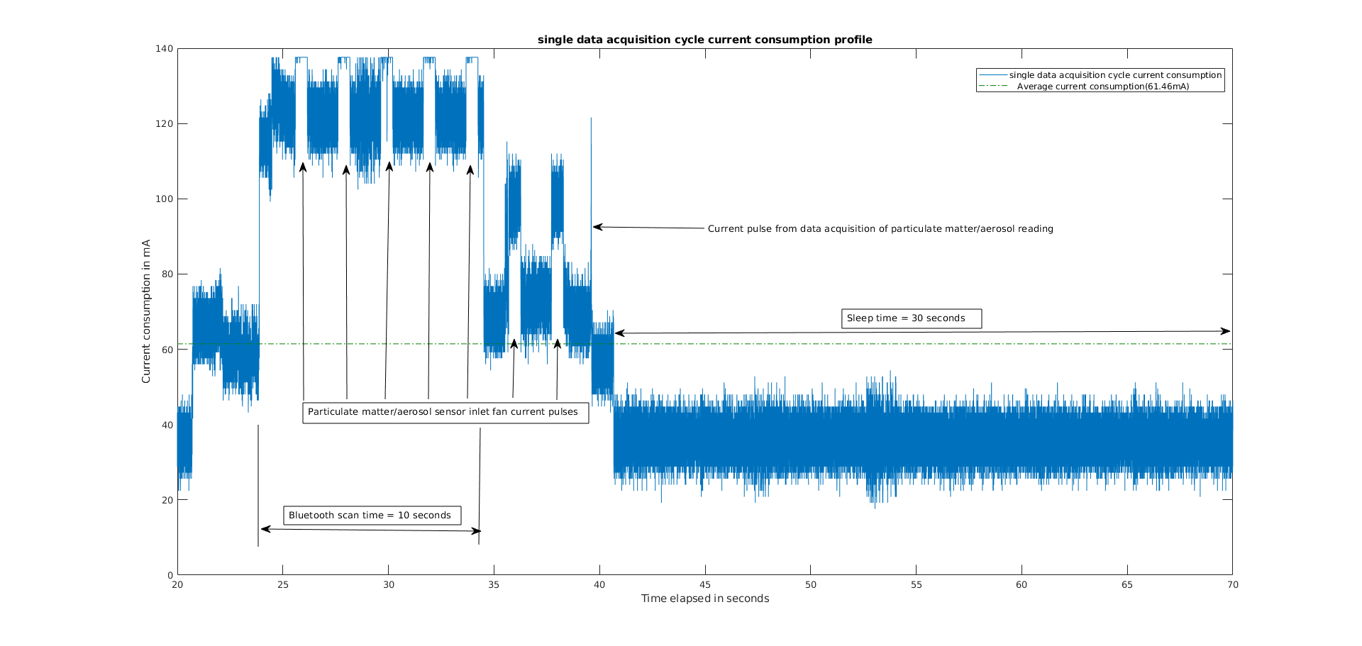
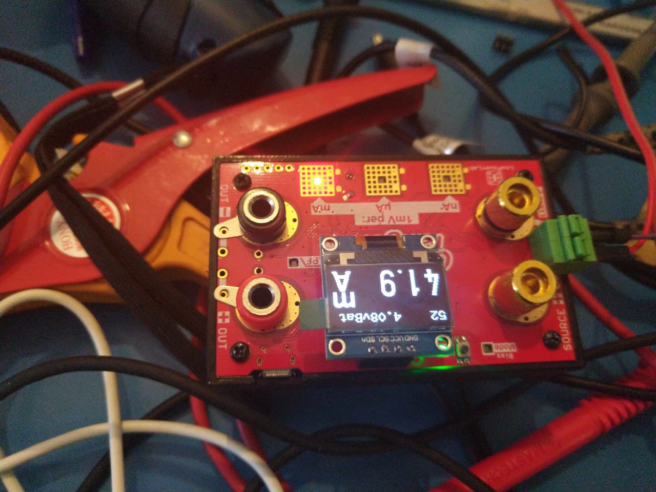
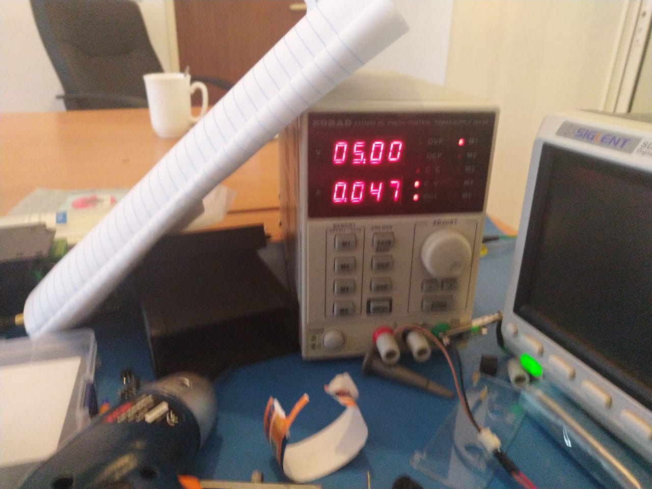
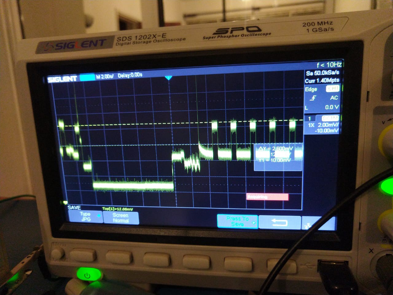
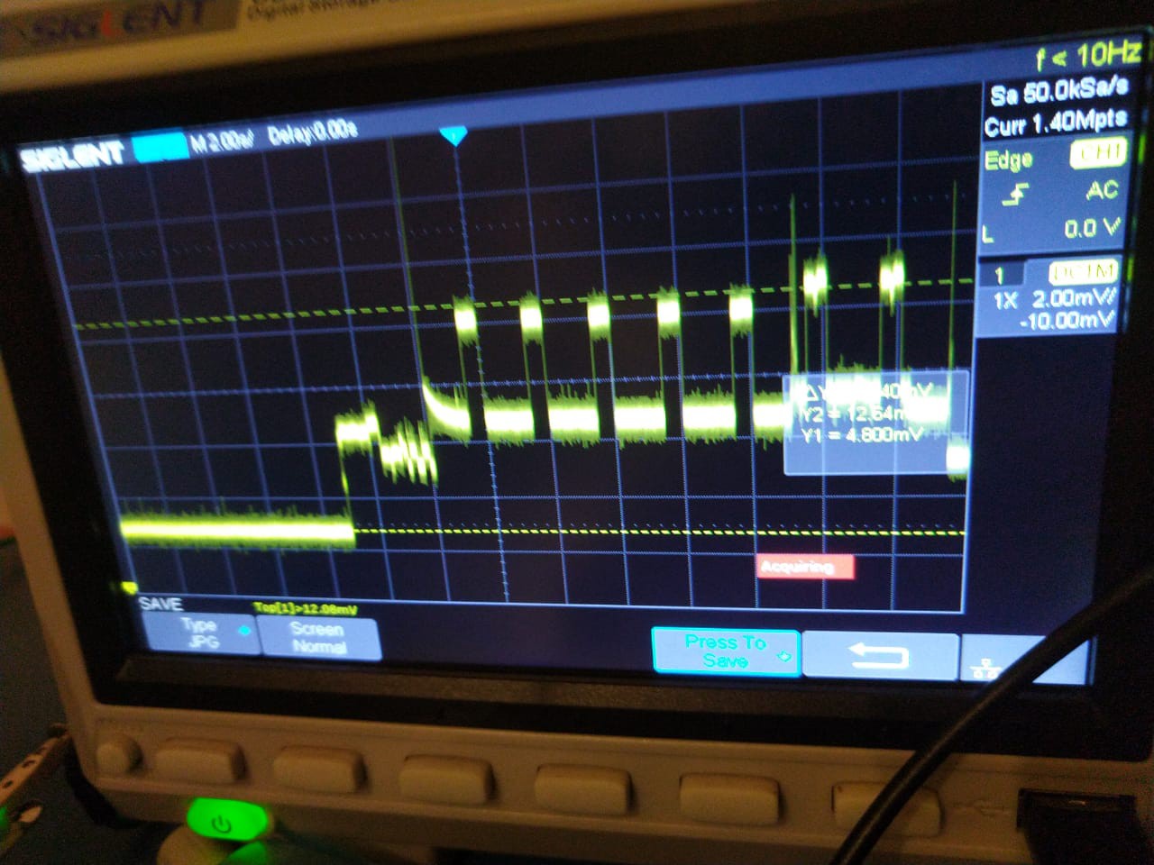
The power consumption of a data acquisition cycle can be seen below.
Power consumption profile(Single data acquisition cycle)
To power profile I used the current ranger with the ground lead replaced with a low noise prong. The data was recorded on an oscilloscope and exported as a CSV for further analysis.
Average power consumption: 61.46mA
Suggested power consumption improvements - Next iteration
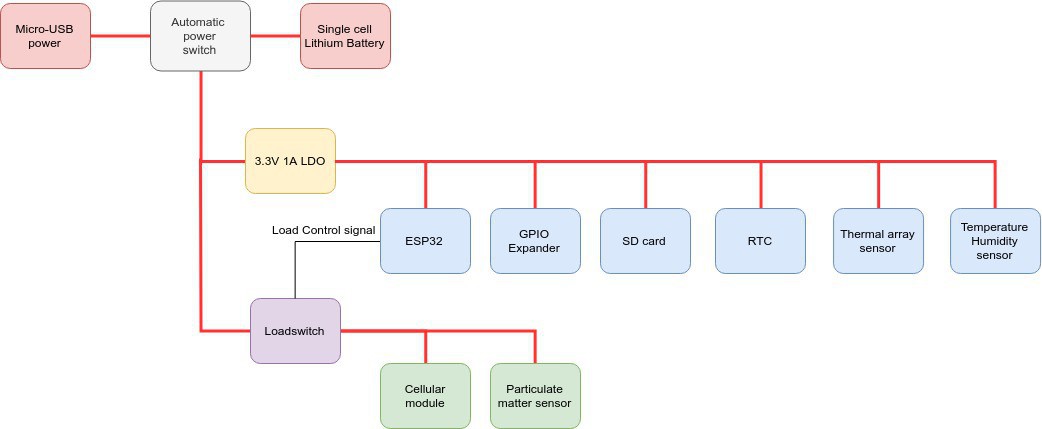
It is noted that the deep sleep phase of the data acquisition phase is around 40 mA. The reason for this may be due to the following factors.
The Particulate matter sensor power mode is software controlled - The datasheet gives a < 10mA idle current.
The load distribution within the system - There are multiple loads on the 3v3 rail that are always active even when the ESP32 is in deep sleep such as:
15-25mA - thermal sensor(20mA)
~10 mA - SD card, RTC, temperature humidity sensor, GPIO expander.
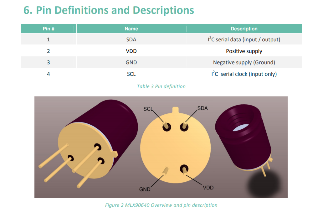
Melexis, creator of the MLX90640 provide a firmware stack that is available directly on github. The stack was written to be run off a Teensy running mbed os. I thus ported the stack over to the ESP-IDF development environment including the test cases with raw data provided with an excel file by the repository maintainer.
The goal is to pass the raw camera parameters through the stack running on the embedded development platform and check that the results are equal to the reference results given by the manufacturer. My forays into doing this is detailed in the project's github issues.
I checked and confirmed the results by comparing the SHA-256 hashes of the reference results against mine, some tests failed and on further inspection, which I suspect to be due to floating point representation and rounding error! I considered this as non impactful!
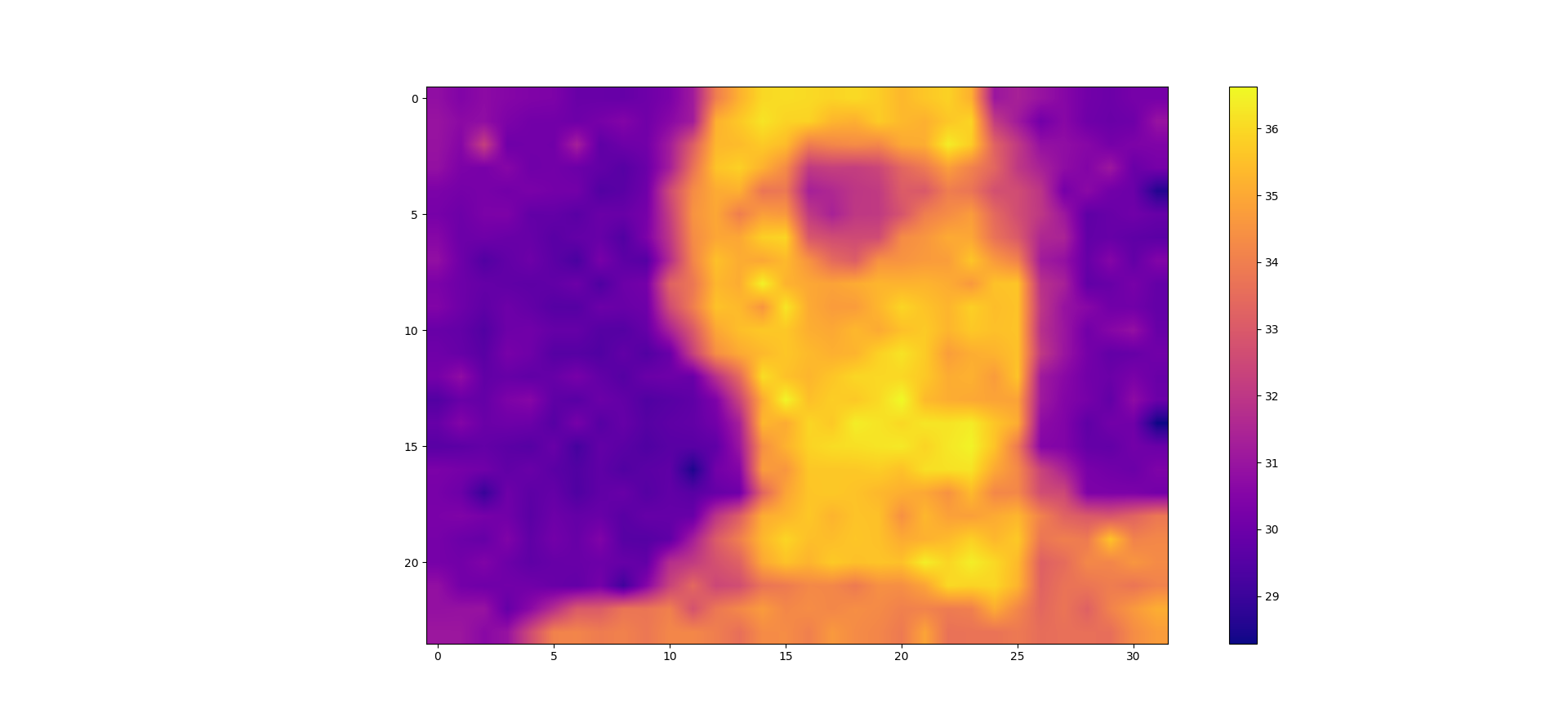
Testing the MLX90640 - Displaying frames
To test that the sensor worked, I printed the raw data of my own thermal representation sent by the thermal camera to the ESP32 processor, to my computer and formatted the data using python as a 2D numpy array(24x32) for plotting. The code is as seen below:
Bilinear interpolated test image of me using the plasma color palette in matplotlib.
A 3D temperature surface plot of a typical thermal image with 24x32 pixels
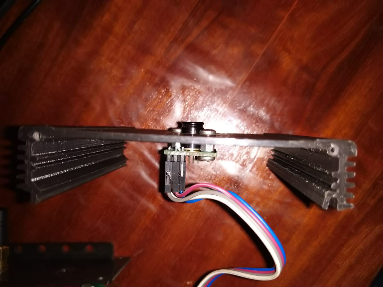
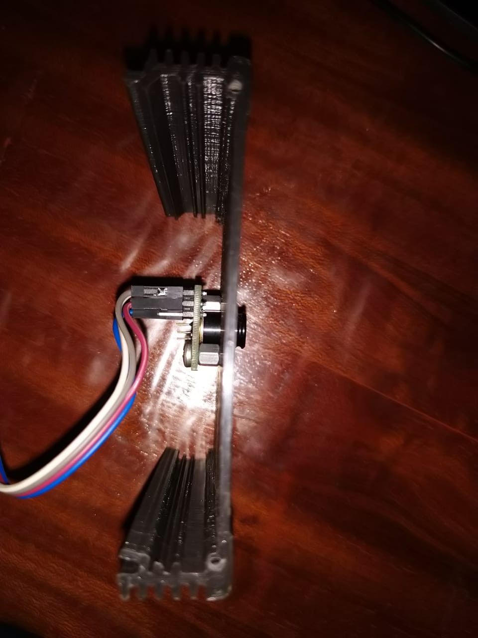
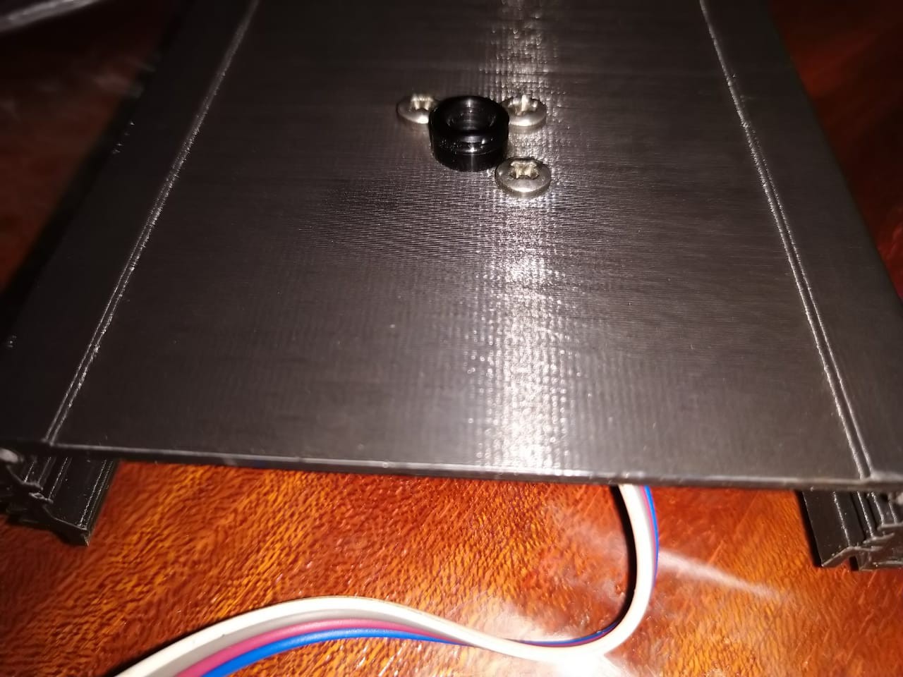
Errata 1: Footprint pinswap - Within the MLX90640 datasheet, the following pins are shown from bottom view. I ported the pins to footprint(Top view) without swapping the view of the pins within the datasheet. The end effect of this is that for the board to work, the top layer had to become the bottom when mounting- Luckily this change still worked well within the entire mechanical assembly without conflicts. Though this would mean the IDC connector would not work as expected as noted in Errata 2.
MLX90640 datasheet pin out
Top layer(Meant to face the Item in view of the MLX90640)Corrected board.
Corrected board.
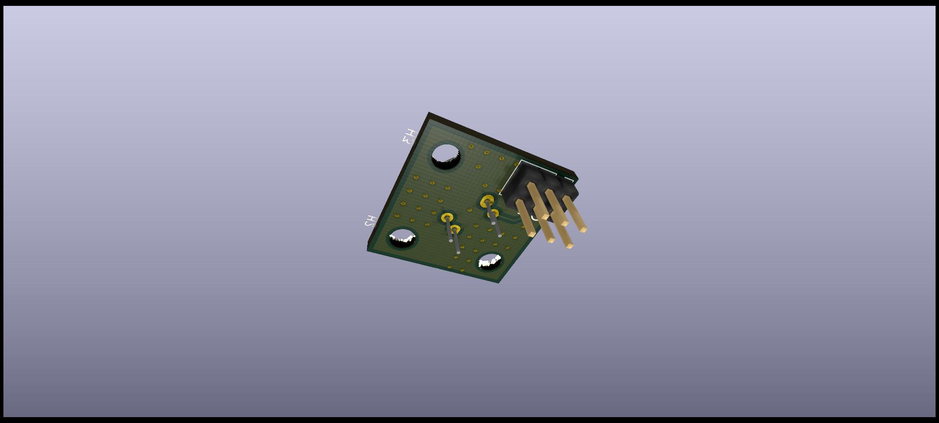
Errata 2: Due to the above errata 1, the 6 pin connector was swapped left-right/right-left due. The problem was remedied by using Female-Female jumpers instead of the desired 6 pin IDC cable. The design flaw can be seen below.
Footprint on add on board(bottom layer in layout).
Footprint on the top layer on the main board
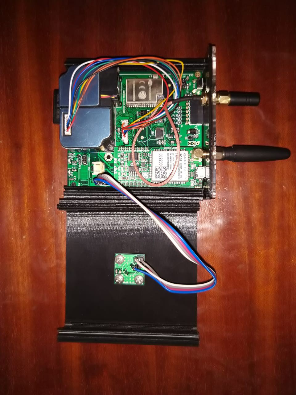
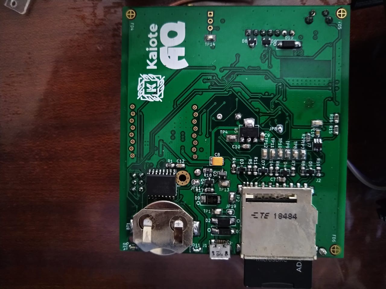
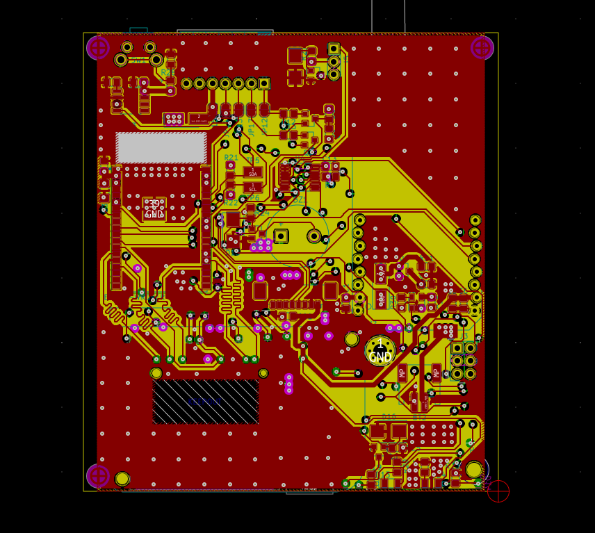
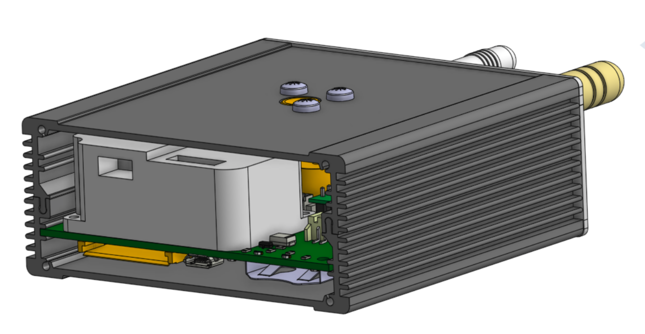
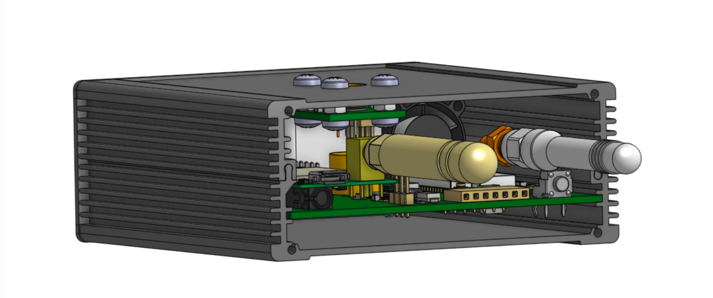
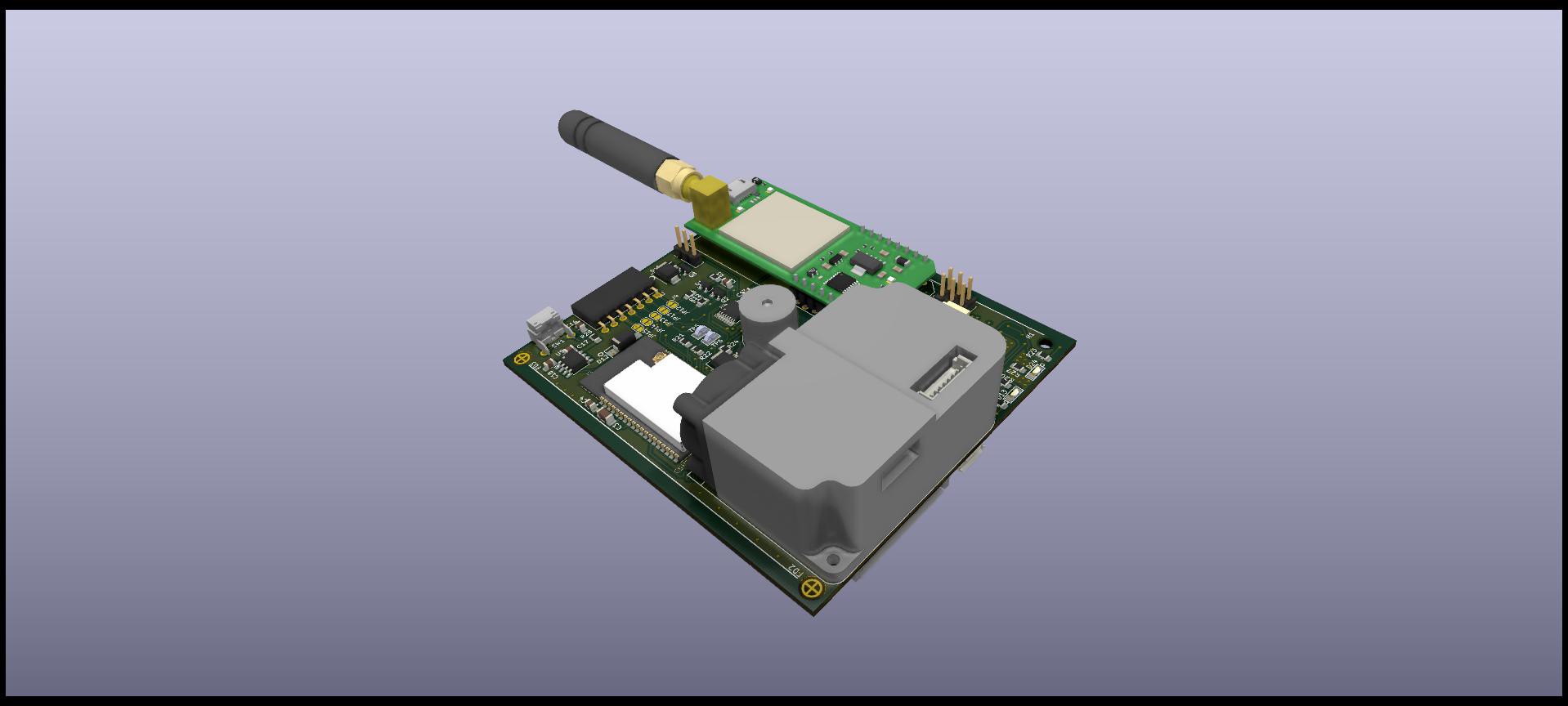
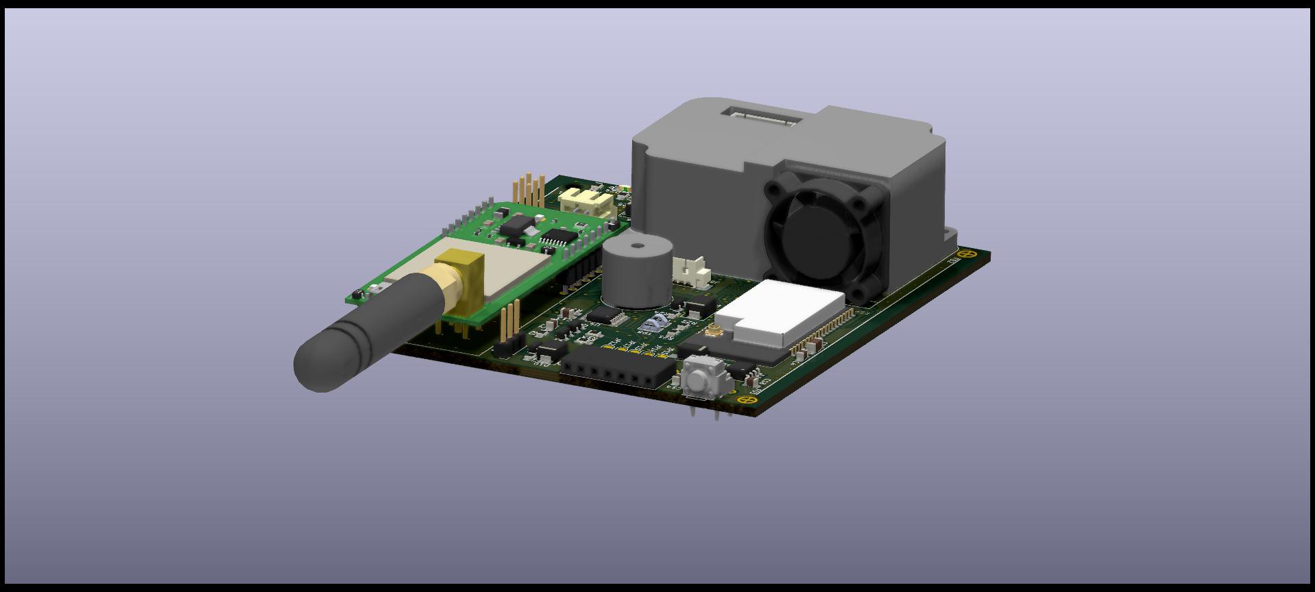
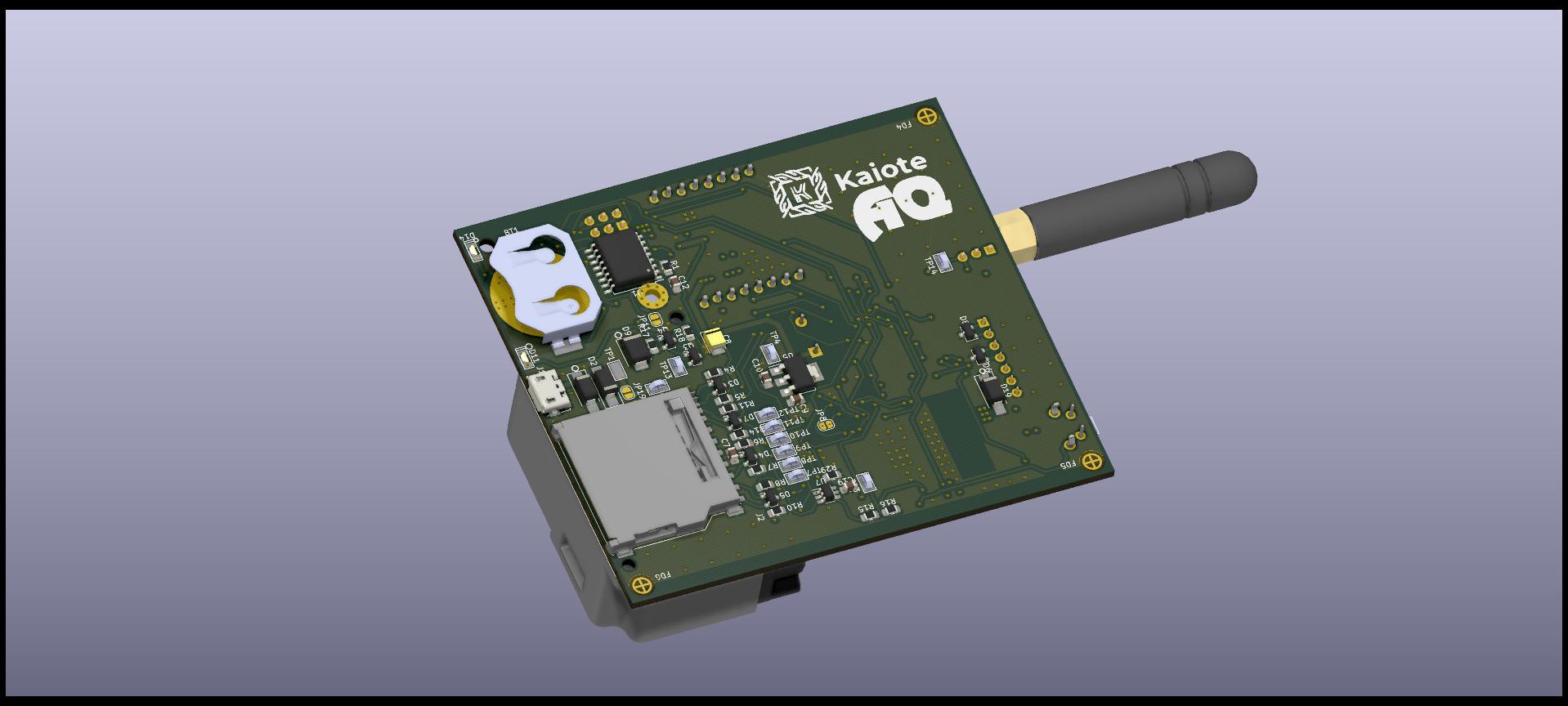
Assembling the main board
Cellular module
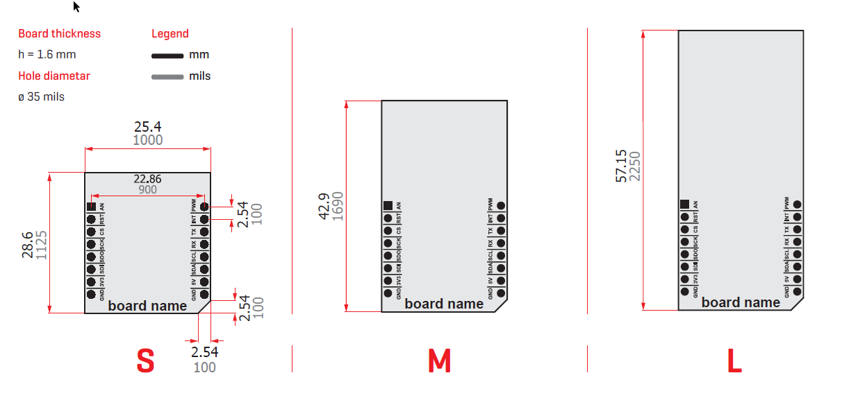
In order to have the ability to swap in and swap out various communication modules based on the Mikrobus footprint standard, the pins were staggered to allow a solderless connection. Each pin was moved off center alternating at 8 mils distance.
The above was ideal because the module chosen followed the Mikrobus open standard, it could easily be swapped out with another. Mikoelektronika has a whole list of Mikrobus modules. This allows one to choose between the following modules:
Note: as at a version 1 on the hardware level, only cellular is possible as I only implemented the UART(TX/RX) and power portion of the Mikrobus standard.
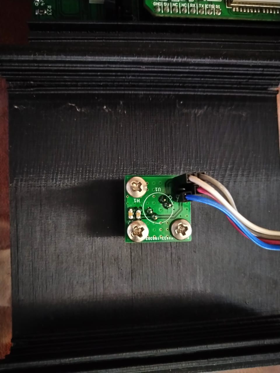
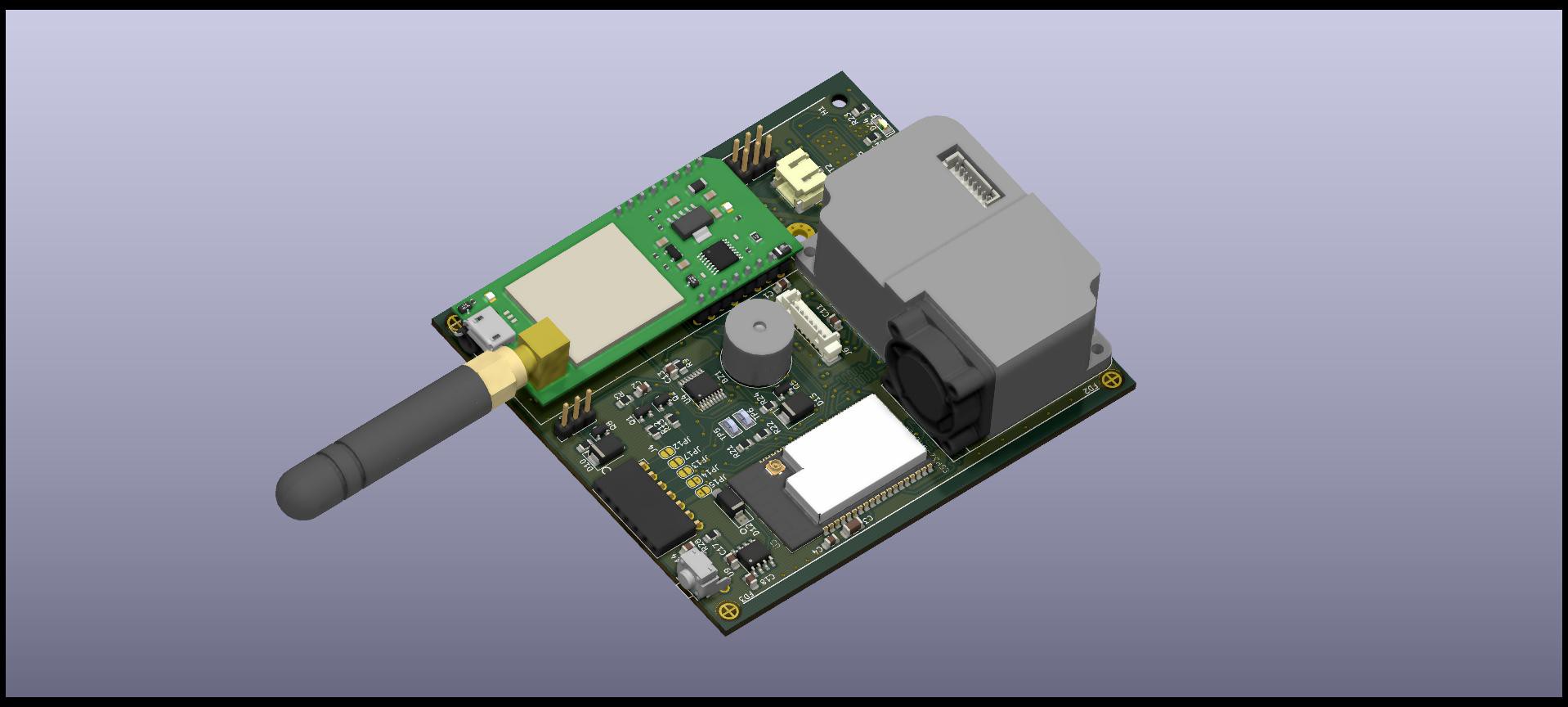
Particulate matter sensor
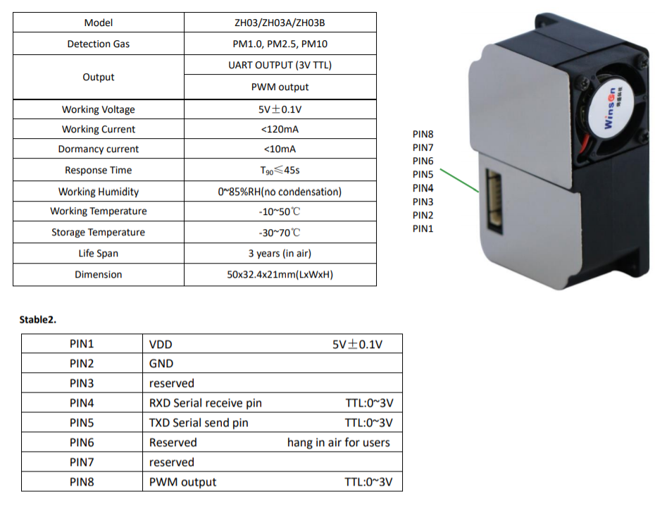
For the particulate matter sensor I used the ZH03B from Winsen electronics. Though the calibration for these sensors are not traceable, the thought is that low cost sensors can be used to show a decrease in pollutant exposure over time as opposed to being used for absolute point measurements.
The ZH03B part did not have a 3D model, I thus created the 3D model in onshape for all variants of the part which include the ZH03, ZH03A and ZH03B. The 3D STEP models can be downloaded from grabcad.
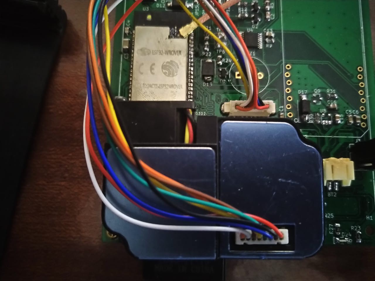
The connector to be placed on the PCB that integrates this sensor is the Boom Precision Elec 1.25T-8P with part number C53040. The Molex picoblade series part number 0533980871can also be substituted for the Boom precision part. Do note the connector is shrouded,thus polarised, therefore you cannot rotate it 180 degrees in case the electrical connections are swapped during design unless by physical removal of one of the shroud walls after PCB placement.
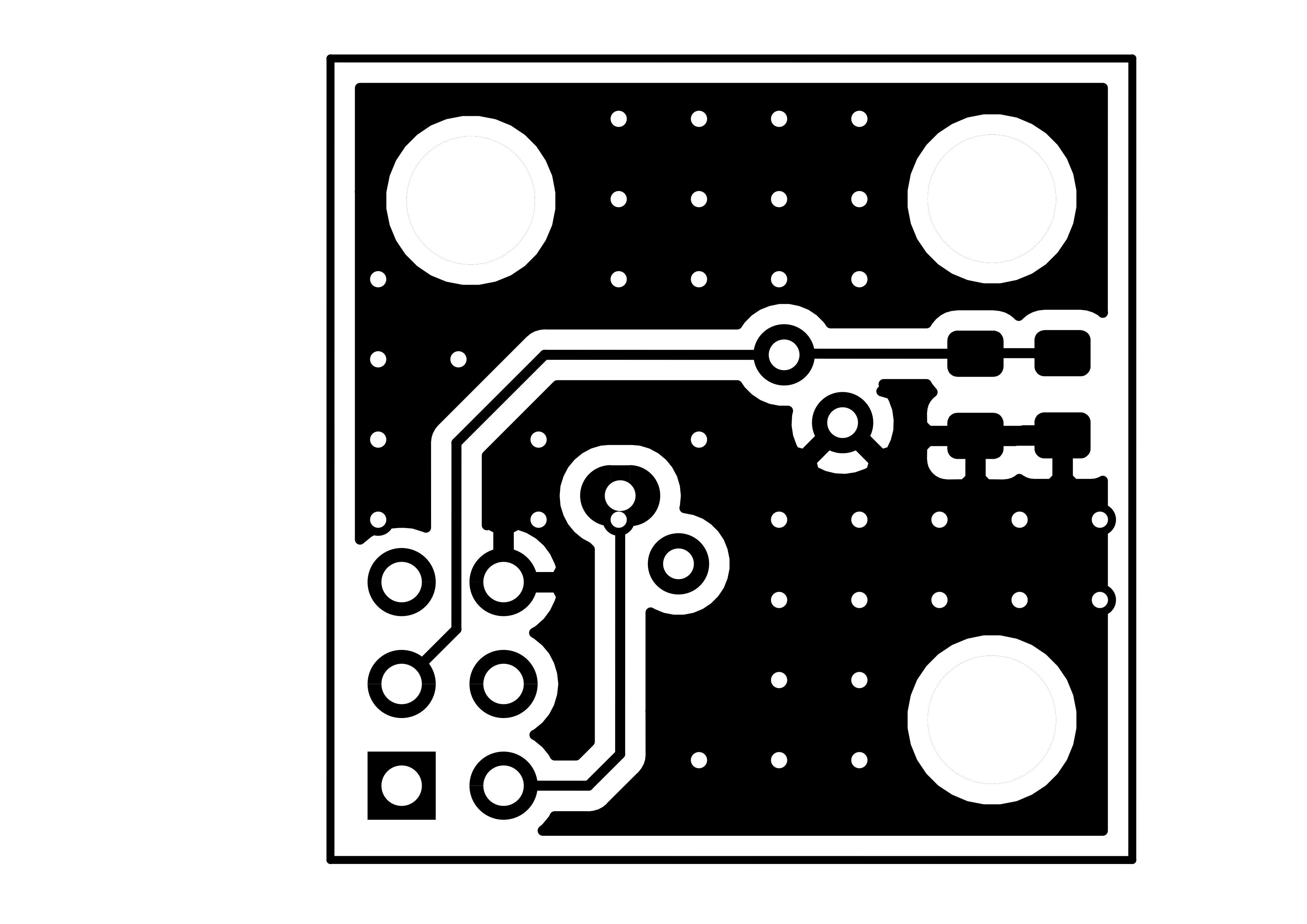
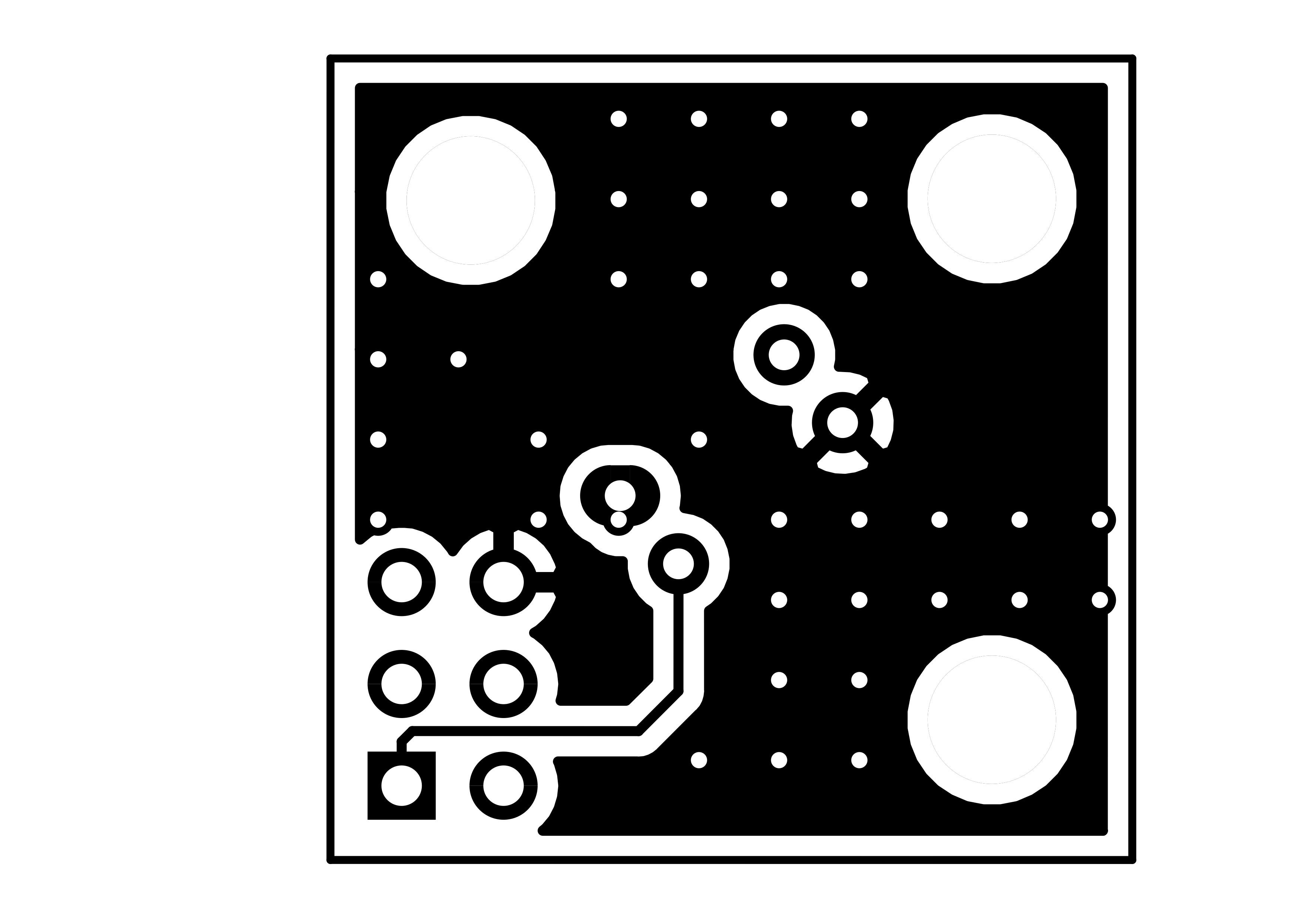
Errata 3: wrongparticulate matter sensor placement-rotated 180 degrees-As can be seen below the footprint pinout was swapped in footprint design. Meaning that Pin 8 on the sensor would be connected to Pin 1 on the main board connector and so on. The remedy was to remove the shroud on the connector, meaning I could invert the cable 180 degrees.
ZH03B pinout
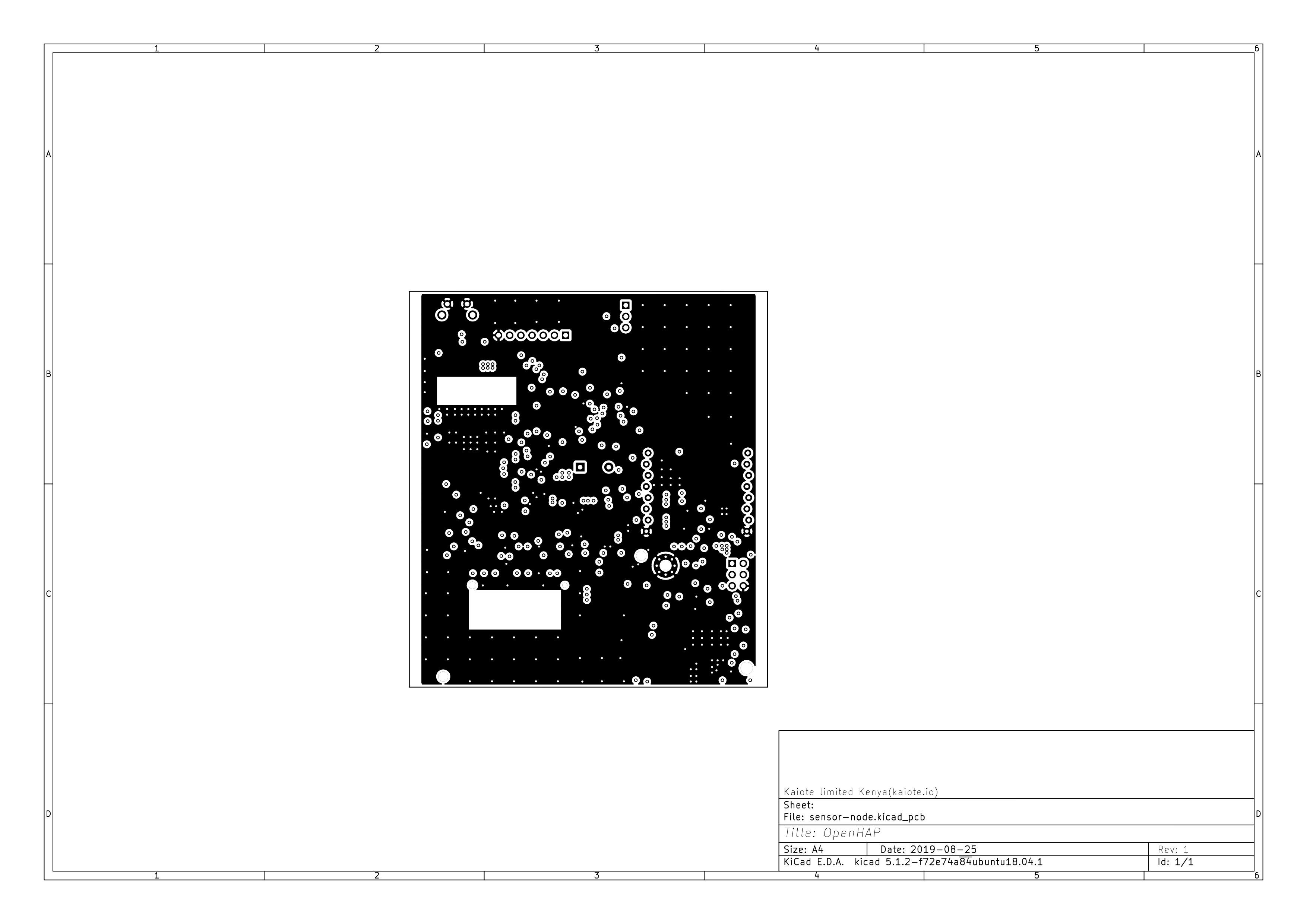
Main board top layer view
Corrected
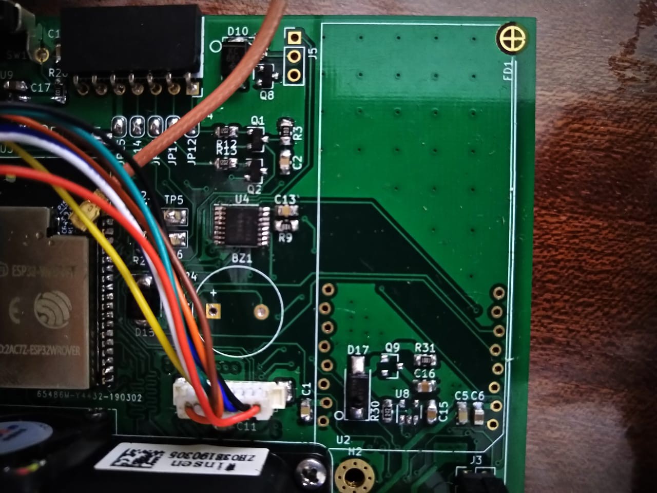
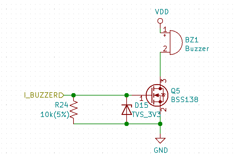
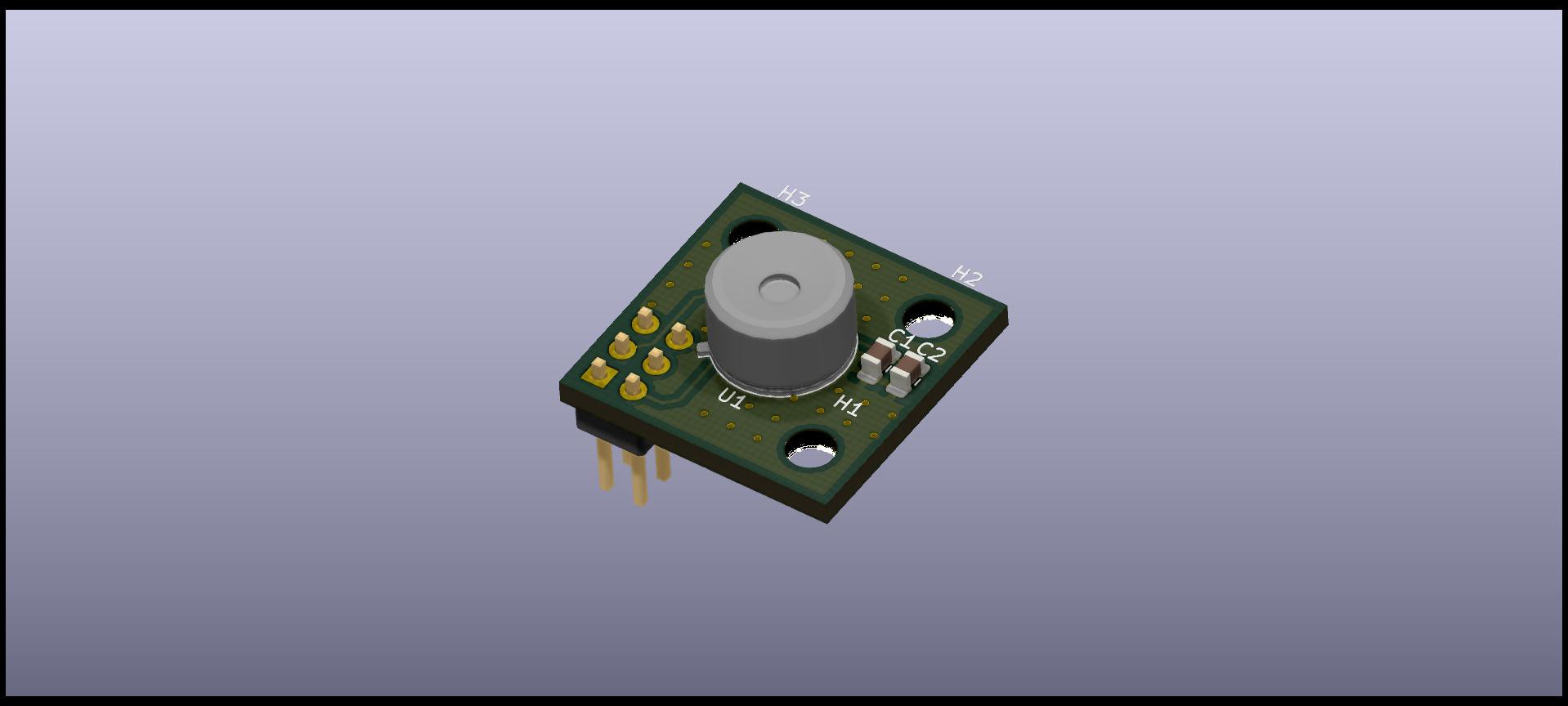
Buzzer
Errata 4: Wrong buzzer selection: The wrong buzzer was selected. Within my schematic, I designed for a self excited buzzer(Constant frequency - usually 2 kHz) but when doing the ordering I chose an externally excited buzzer that required an external oscillator circuit to drive it!(Varying audible frequency as a result)
As we needed to test the enclosure fitting prior to choosing extruded aluminum, we settled for 3D printing as we could get our prints with a 2 day lead time. We chose Cubic 3D as our printing partner. They offer affordable printing services in Kenya and have very good customer service. Quite impressive considering that the printing service is lead by 2 undergraduate students.
On login, we uploaded our 3D prints.
Total cost for a single unit(all parts combined) came to 11 USD.
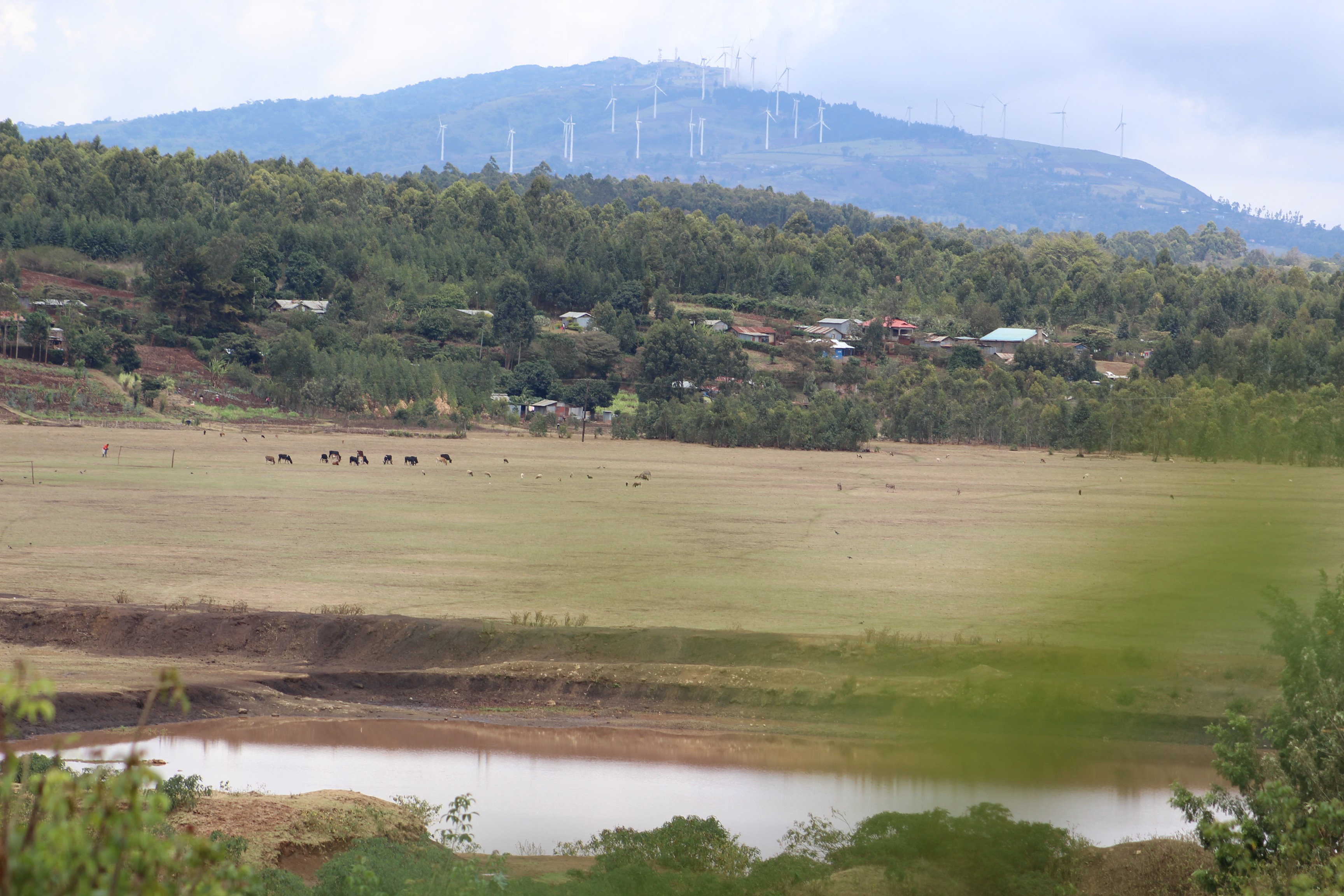
Is state of household air pollution really that bad?- This is the question I doubtfully asked myself in March 2019 while doing research on the problem above as I was designing an household air pollution monitor for a study being carried out by EED Advisory for SNV, the Dutch development agency on the cooking the sector in Kenya.
Nothing could have prepared me for the truth as my first openHAP field test did in rural Kenya.
The rural area in Kiambu county, Kenya. In the background are Ngong hills and its wind farm. The air looks so clean doesn't it?
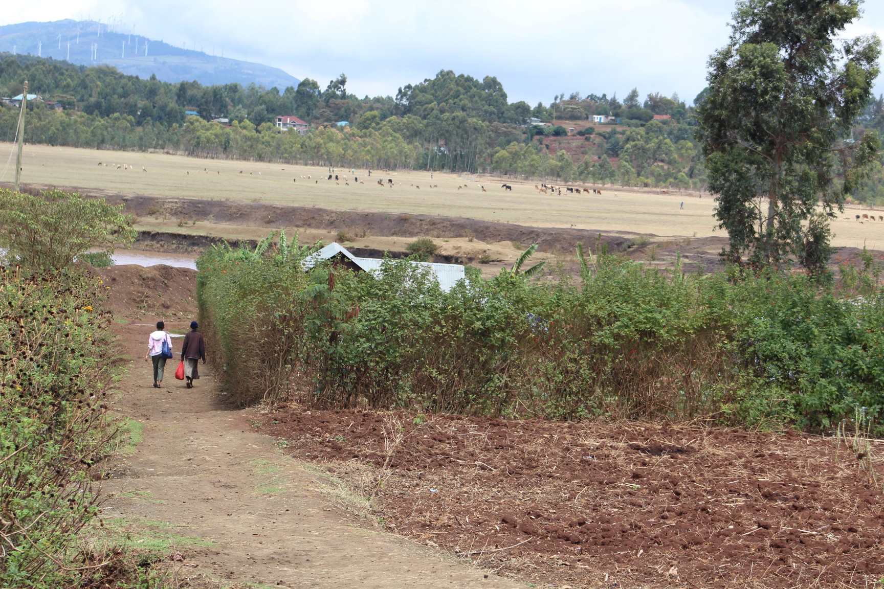
The home that we were welcomed to visit take sample measurements. The lady who welcomed us so nicely can be seen in the distance with my colleague.
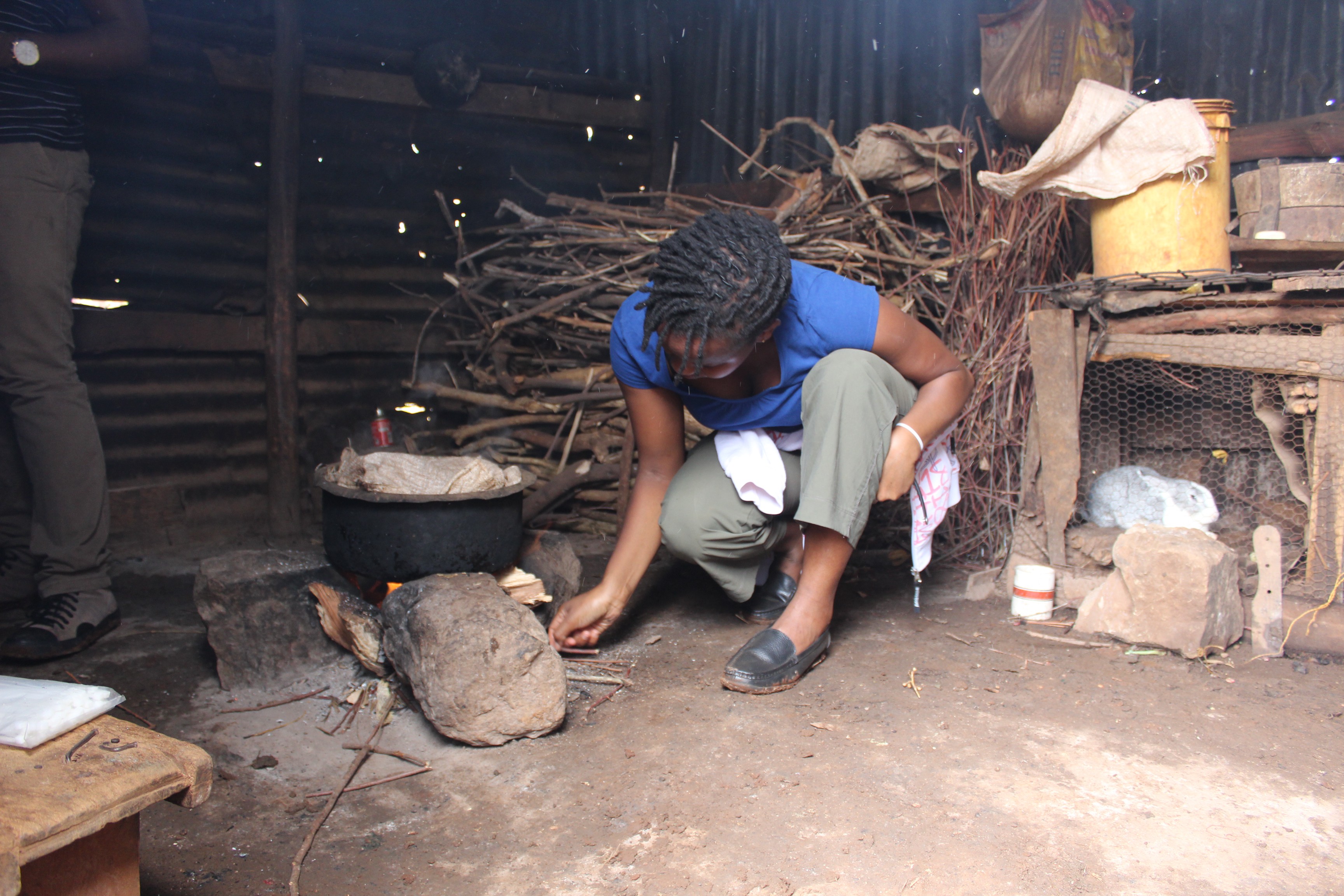
The home uses a Three stone open fire(TSOF) stove which is one of the most widely available stoves globally due to the ease of building materials and the minimal skills needed. Details are well documented here.
An illustration of a Three Stone Open fire(TSOF) stove taken from the Improved cookstoves training manual, hosted within the Humanity Development Library 2.0 by the Humanities Library Project.
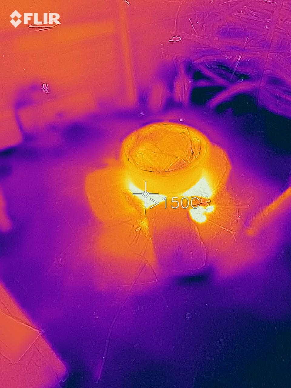
Stove temperatures as seen on a FliR Thermal camera
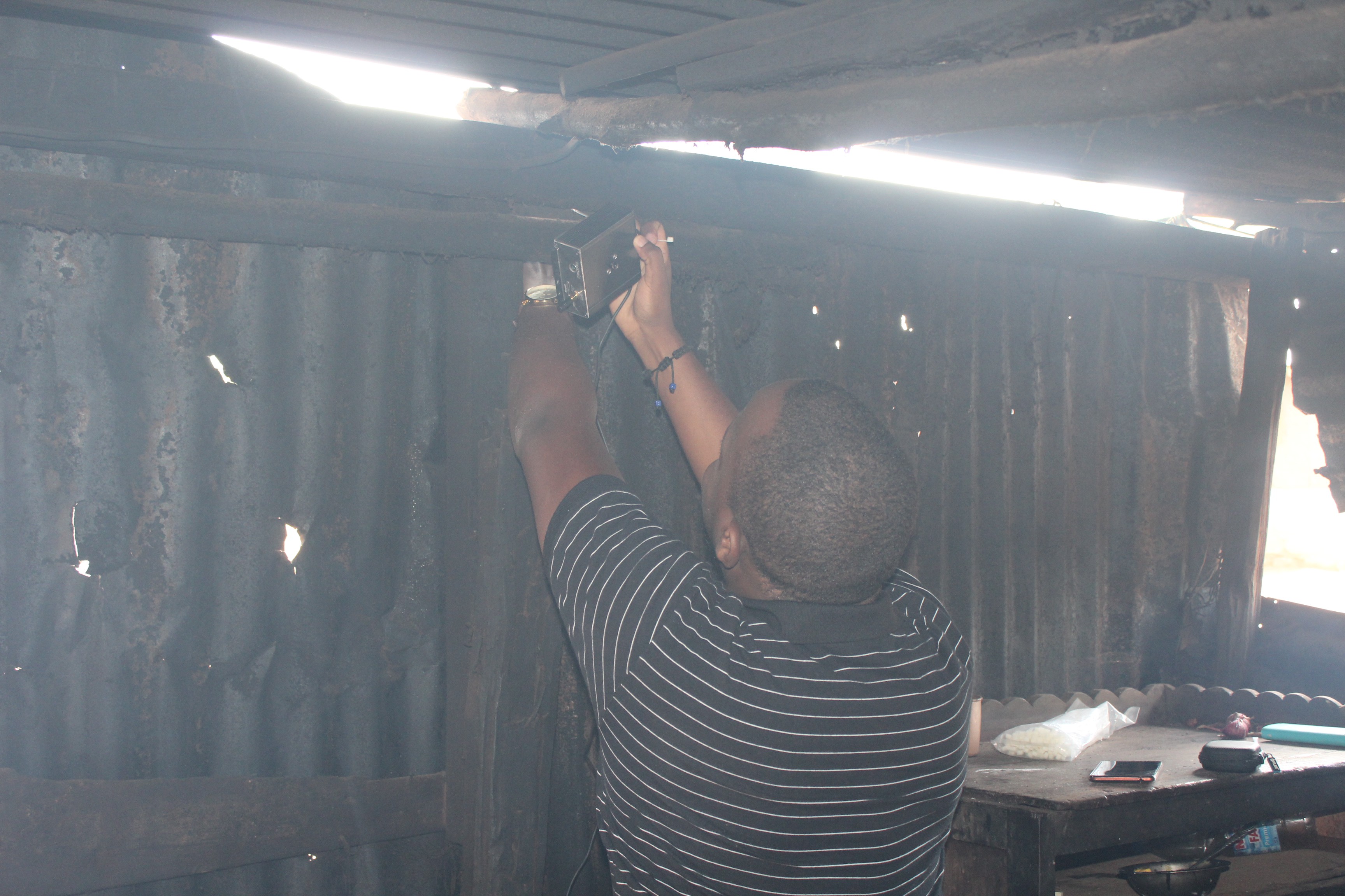
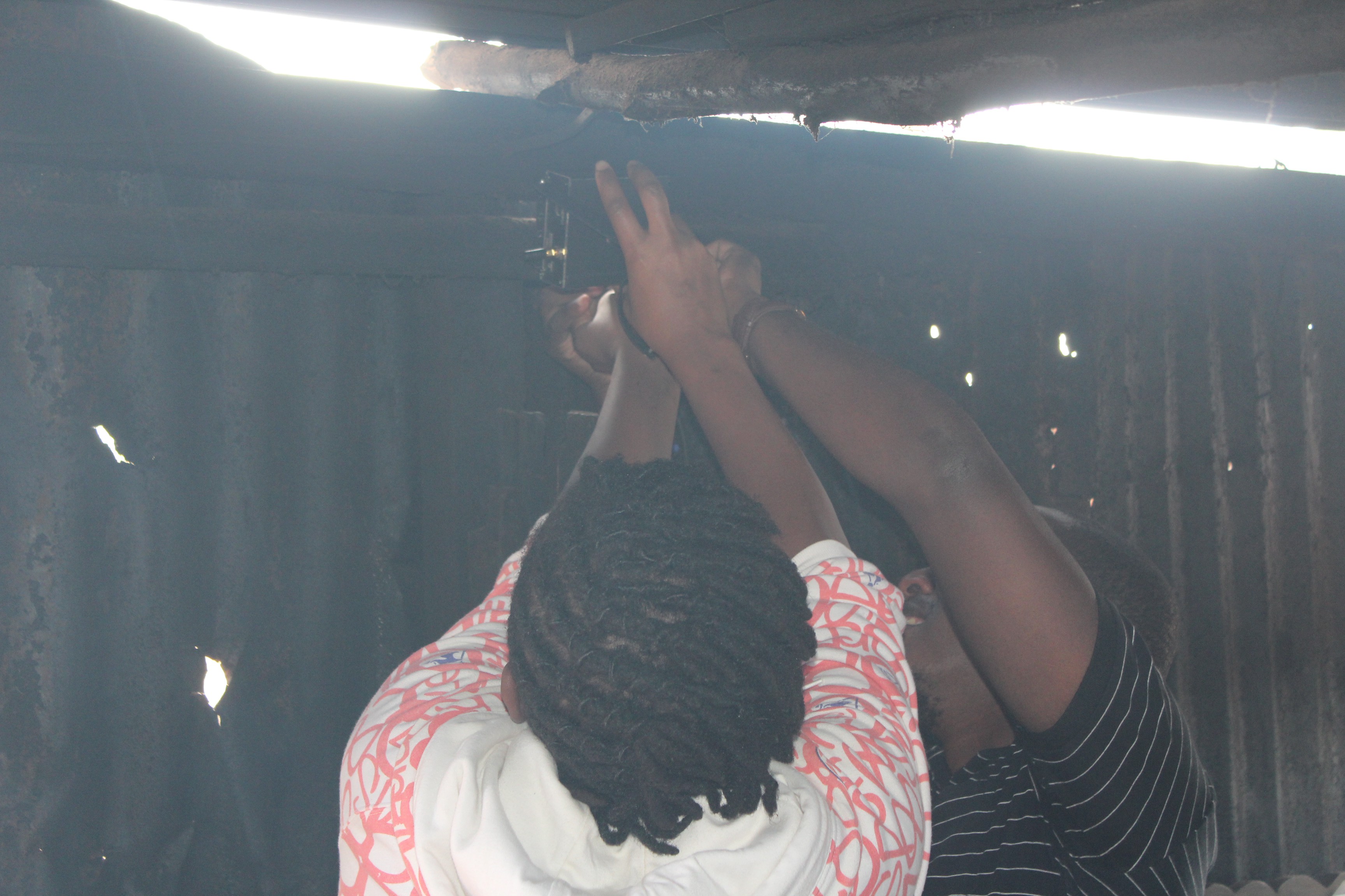
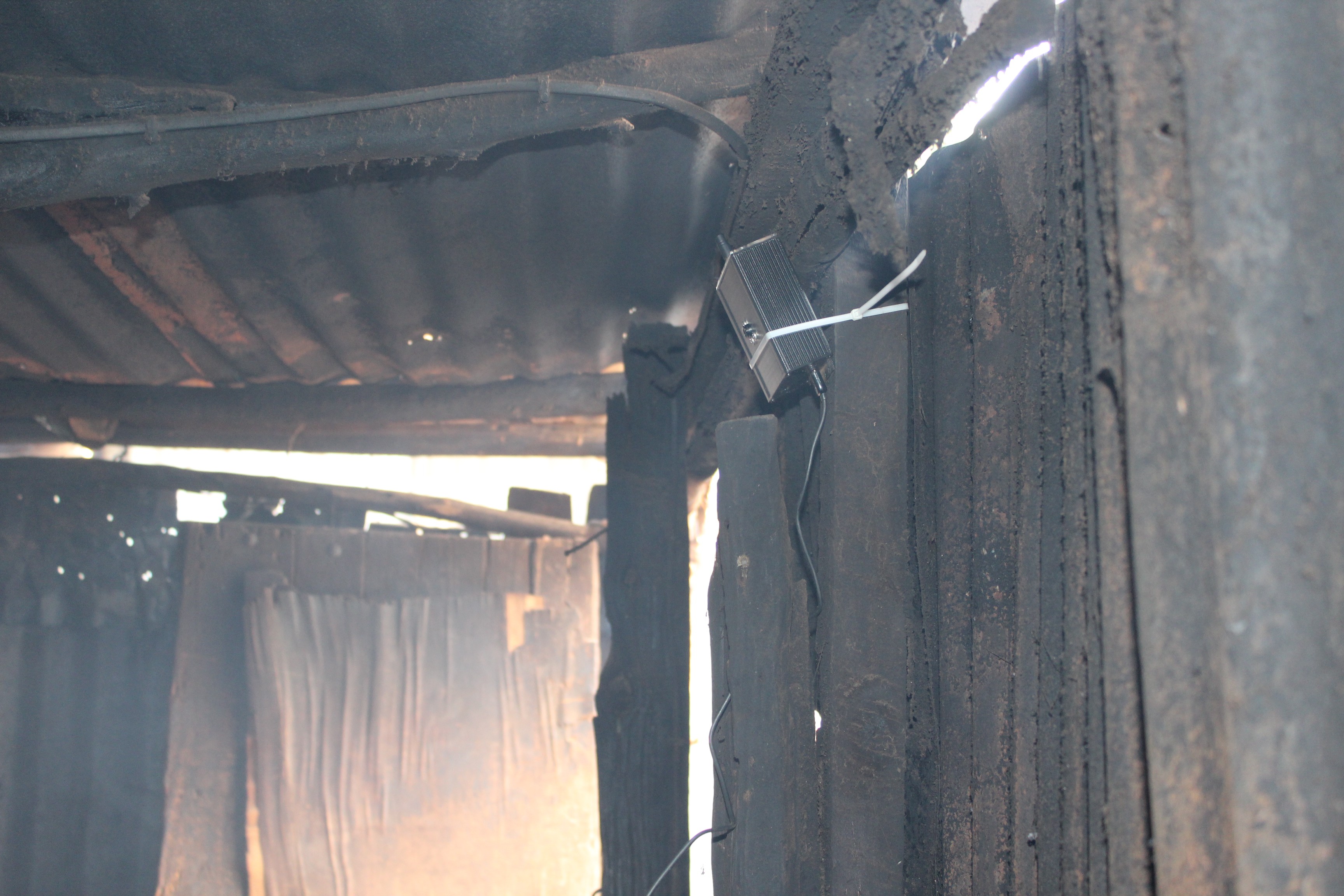
The mock cooking exercise started as soon as I began setting up the openHAP prototype unit. Though the camera does not capture the smoke levels well, the build up much faster than anticipated as it took less than just 30 seconds by my approximation for it to reach the point I couldn't see. At that moment the closest thing I could compare it to was industrial flue gasIndustrial flue gas emissions"Help me, I cant see!" By this time everybody except us had vacated the kitchen due to the smoke, even the lady who invited us could only just watch our brave efforts from outside,"Help me, I cant see!" By this time everybody except us had vacated the kitchen due to the smoke, even the lady who invited us could only just watch our brave efforts from outside,The prototype OpenHAP unit already setup. One can see the thick layer of soot coating formed on the corrugated iron sheets over time. It is still unbelievable how the lungs and eyes can take such a beating for so long given that people cook three times a day and this kitchen has been here for years!After 48 hours, we downloaded the data from the OpenHAP prototype unit and analysed it. Apparently the readings were so high that it exceeded the upper detection threshold of our particulate sensor! From the calculations, the lady who invited us(primary participant in the graph) was taking in the equivalent of 8 cigarettes a day and approximately 8 times above WHO's 24 hour exposure limit just based on our curtailed particulate matter sensor readings.
After testing the unit in rural Kenya and seeing the data, we decided to open source the openHAP design and methodology and give support to its development through our subsidiary, Kaiote as a public domain project allowing others to make copies and derivatives.
Is household air pollution really that bad?- This is the question I doubtfully asked myself 3 months ago while doing research on the problem above as I was designing an household air pollution monitor for a study being carried out by EED Advisory for SNV, the Dutch development agency on the cooking the sector in Kenya.
Nothing could have prepared me for the truth as my first openHAP field test did in rural Kenya.
The rural area in Kiambu county, Kenya. In the background are Ngong hills and its wind farm. The air looks so clean doesn't it?
The home that we were welcomed to visit take sample measurements. The lady who welcomed us so nicely can be seen in the distance with my colleague.
The home uses a Three stone open fire(TSOF) stove which is one of the most widely available stoves globally due to the ease of building materials and the minimal skills needed. Details are well documented here.
An illustration of a Three Stone Open fire(TSOF) stove taken from the Improved cookstoves training manual, hosted within the Humanity Development Library 2.0 by the Humanities Library Project.
Stove temperatures as seen on a FliR Thermal camera
The mock cooking exercise started as soon as I began setting up the openHAP prototype unit. Though the camera does not capture the smoke levels well, the build up much faster than anticipated as it took less than just 30 seconds by my approximation for it to reach the point I couldn't see. At that moment the closest thing I could compare it to was industrial flue gasIndustrial flue gas emissions"Help me, I cant see!" By this time everybody except us had vacated the kitchen due to the smoke, even the lady who invited us could only just watch our brave efforts from outside,"Help me, I cant see!" By this time everybody except us had vacated the kitchen due to the smoke, even the lady who invited us could only just watch our brave efforts from outside,The prototype OpenHAP unit already setup. One can see the thick layer of soot coating formed on the corrugated iron sheets over time. It is still unbelievable how the lungs and eyes can take such a beating for so long given that people cook three times a day and this kitchen has been here for years!After 48 hours, we downloaded the data from the OpenHAP prototype unit and analysed it. Apparently the readings were so high that it exceeded the upper detection threshold of our particulate sensor! From the calculations, the lady who invited us(primary participant in the graph) was taking in the equivalent of 8 cigarettes a day and approximately 8 times above WHO's 24 hour exposure limit just based on our curtailed particulate matter sensor readings.
After testing the unit in rural Kenya and seeing the data, we decided to open source the openHAP design and methodology and give support to its development through our subsidiary, Kaiote as a public domain project allowing others to make copies and derivatives.
 aloismbutura
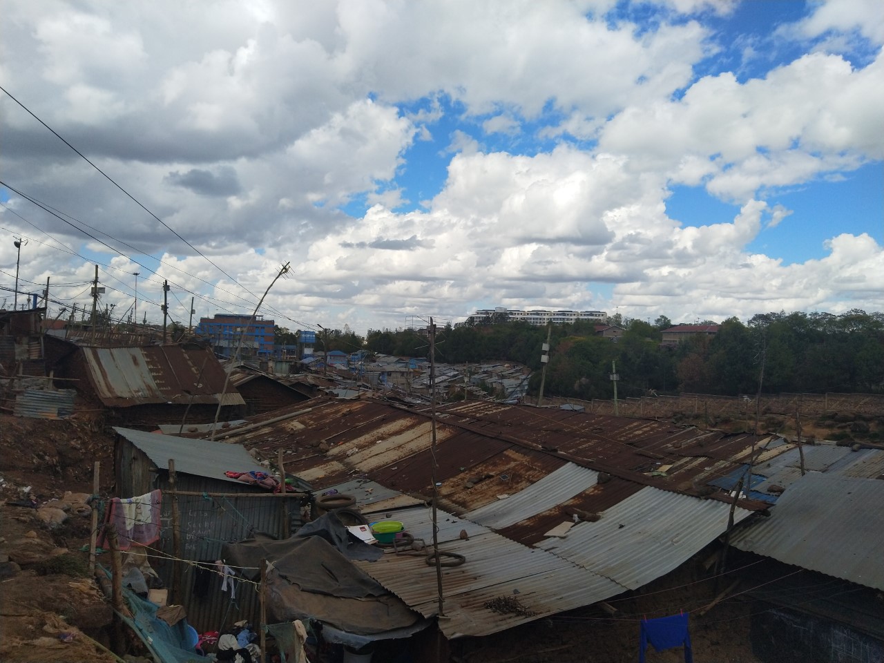

 A sample briquette stove