The goal of this task is to describe the steps needed to translate a neural network onto a discrete component implementation

Sample neural network

As a starting point we'll use a simple neural network with two inputs or signals and two outputs or classes. In the MNIST example, each input would be a sensor on the 4x4 matrix and the outputs or classes would be digits from 0-9.

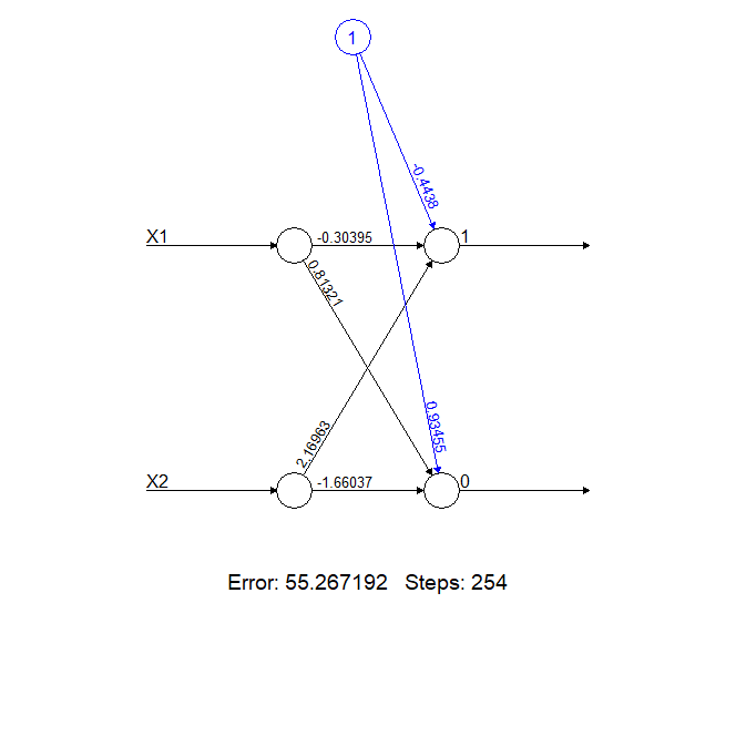
In the image below we have a neural network composed of two neurons, identified as 0 and 1. Since this neural network has no hidden layers, the output neurons are the only neurons.

The calculations carried out at the neurons are as follows:

• Neuron 1 = Bias (-0.4438) + Input X1 * weight_X1_1 (-0.30395) + Input X2 * weight_X2_1 (2.16963)
• Neuron 0 = Bias (0.93455) + Input X1 * weight_X1_2 (0.81321) + Input X2 * weight_X2_2 (-1.66037)

We'll now translate this onto a memristor as follows:

• Each neuron's (0 or 1) signal will be calculated as a summation of currents
• The bias term will be translated onto a current (positive or negative).
• The Input * weight terms will be translated onto currents (positive or negative).
• All the terms will be channeled onto a wire and the summation current will be transformed onto a voltage signal using a resistor. The signal will vary in intensity with the increasing current across the neuron.

Positive value currents will be simply calculated as the product of the incoming voltage and conductance of a resistor (I = V x G or I = V / R). The resistor has to be chosen so that the conductance of the resistor equals the value of the weight. For example, in the neural network above, for Sensor X1 and the Output signal 0, the weight equals 0.81321 and the equivalent resistor would have a resistance of 1.2 ohms. The resulting current will be injected into the neuron wire.

Negative value currents will be calculated by multiplying the incoming voltage by a suitable resistor. The resulting negative current will be subtracted (removed) from the neuron line using a transistor. The resistor has to be chosen so that the conductance of the resistor equals the weight divided by the beta of the transistor. For example, in the neural network above, for sensor X1 and the output signal 1, the weight equals -0.30395. Assuming the transistor has a beta of 100, the resistor would have to be (0.30395/100)^-1 = ~300 ohms. There is a better way to do this and this was suggested by the vibrant community in the .Stack in order to avoid the impact of beta variation as a function of Collector current. We'll stick to this simpler solution for now and discuss the alternative implementation below.

Finally, the bias in neuron 1 is a negative one. Hence we need to use the transistor to subtract current from the neuron line. The value for the bias is -0.4438. Using the same procedure as above, we'll calculate the resistor value as (0.4438/100)^-1 = 225 ohms.

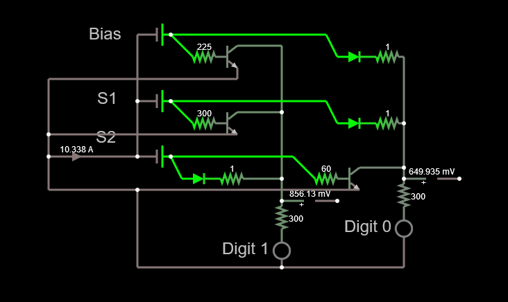
Adding it all up

In order to add the currents and get the output of the neuron, we use a wire joining all the currents and display the signal as intensity of a led. We could also measure the voltage with an ADC if we wanted to handle the output digitally.

The resulting circuit is simple, if slightly dangerous if we pay close attention to the ammeter below the S2 signal. The reason for this is the amount of sensors. Since the number of sensors is small and the data poor, we are stuck with very large weights and biases. This means that if we move the sliders controlling the voltage from the sensors to their maximum values, we get currents in the order of a few amperes. When scaling up to as little as 16 pixels/sensors, this is not the case anymore and the weights and biases are much smaller. We'll tackle this issue later.

An improved negative weight calculation

Since the beta of the transistors is not a reliable number, I asked the .Stack to lend a hand to try to solve the issue caused by its variation. I got a lot of useful information. One answer led me to log this log, but all of them sent me on a way to solve the issues caused by the variability of beta.

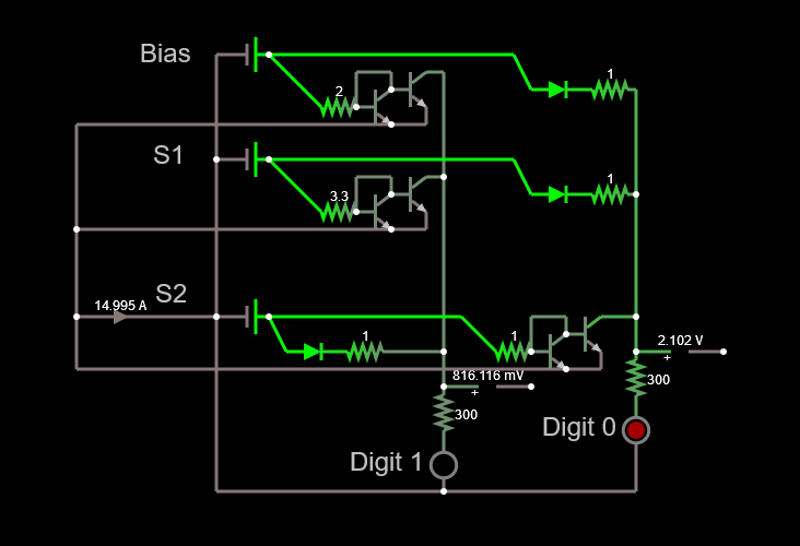
Darrin B suggested using a current mirror instead of single transistor and that helped me to solve the beta issue. The updated circuit can be seen below.

So, now the issue with the beta is solved, but we still have a 14.9 A current to deal with.

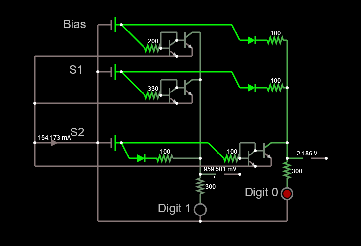
Since we're looking at the comparative signals between 0 and 1, we can in principle massage the maths as follows and still maintain the ratio between the two signals:

• Neuron 1 = Bias (-0.4438) / 100 + Input X1 * weight_X1_1 (-0.30395) / 100 + Input X2 * weight_X2_1 (2.16963) / 100
• Neuron 0 = Bias (0.93455) / 100 + Input X1 * weight_X1_2 (0.81321) / 100 + Input X2 * weight_X2_2 (-1.66037) * 100

We then end up with the circuit below, which has a much higher impedance and a more palatable current.

Conclusion

Hopefully this task helps understand the basics of translating a trained neural network onto a discrete component affair.

There were some issues with the previous circuit design which have been solved with the feedback from the .Stack and some basic math.

The circuit for the MNIST number recognition neural network will be updated using the lessons learned and fingers crossed we'll have a prototype soon.

The goal of this task is to design a PCB that will allow a trained neural network to be used to detect MNIST numbers from an image.

Sensor array and signal selection

During the analysis of the results reported in the previous log, I realised that actually jumping from a 16-pixel sensor matrix to a 49-pixel sensor matrix had two significant effects. The first one was in the design of the sensor array. The second one and even more significant was on the memristor. Considering my limited experience in PCB design, and looking at simulations of the memristor in action, I decided to stick to 4 x 4 matrix using the intensity level from the sensors instead of the binary response. Also because the 7x7 matrix using the model with a binary signal did not perform that well and it had a very significant cost in complexity.

Assuming like I did for the previous model an average of 1.5 components per node for the memristor, and using 49 inputs and 10 outputs, I'd have a whooping 450 components to mount (that'd be for every input, 10 weights and a bias, multiplied by the number of outputs). Anyway, my initial 1.5 component per node was a little bit off as we'll see later.

The attached simulation can be run here and shows that the neural network is quite robust and small changes in some of the sensors do not make a significant difference in the result. Nevertheless, we'll need to test this in real life.

The simulation actually helped me to see a significant issue with the design that I had not predicted. This was quickly solved with a bit of learning about passive components. Shocking as it was for me,  I didn't know electricity could flow backwards.

Memristor design

The initial memristor design needed a bit of math to adjust the negative weights. The positive weights were calculated simply by multiplying the input voltage by the conductance of the resistor, the result being a current.

For the negative weights, I needed to subtract the current, and this was achieved by using an npn transistor that would conduct the current in the base multiplied by beta (I didn't even know this number existed, learning as we go long). So, all things considered, I found out that beta was not constant with the input current.

If anyone knows of a type of transistor that has a beta that has a small variation with current, please send me a comment. I'd really appreciate any help on this.

I tested the impact of a variation in beta in the simulation and found that this was also not very significant on the result of the neural network. Then again, we'll have to test this in real life.

So, my problem appeared when I put an LED at the back of the digit line. In order to see whether it's one digit or the other, I chose to add an LED with a resistor. The problem was that the current in some conditions, chose to flow backwards instead of forward in some conditions. Since the signal is a current, I could not afford losing current to other part of the circuits. This was quickly solved with a diode in line with the input resistor as can be seen in the video below.

This is an incredibly basic concept but up until this time I had never actually needed a diode, nor I knew very well how they worked. That last bit still holds today.

Instead of having nodes with a 1.5 average component count, I had now two. Initially the nodes with positive bias had a resistor and the ones with negative bias a resistor and a transistor. In big numbers average 1.5. Now I had a diode and a resistor for the positive bias and a resistor and a transistor for the negative bias. Total count was now 16 inputs , 1 weight per input plus a bias for each multiplied by 10 outputs, 2 components per node. Theoretical part count 340. The actual value came a little bit higher due to connectors and LEDs, but close to the mark.

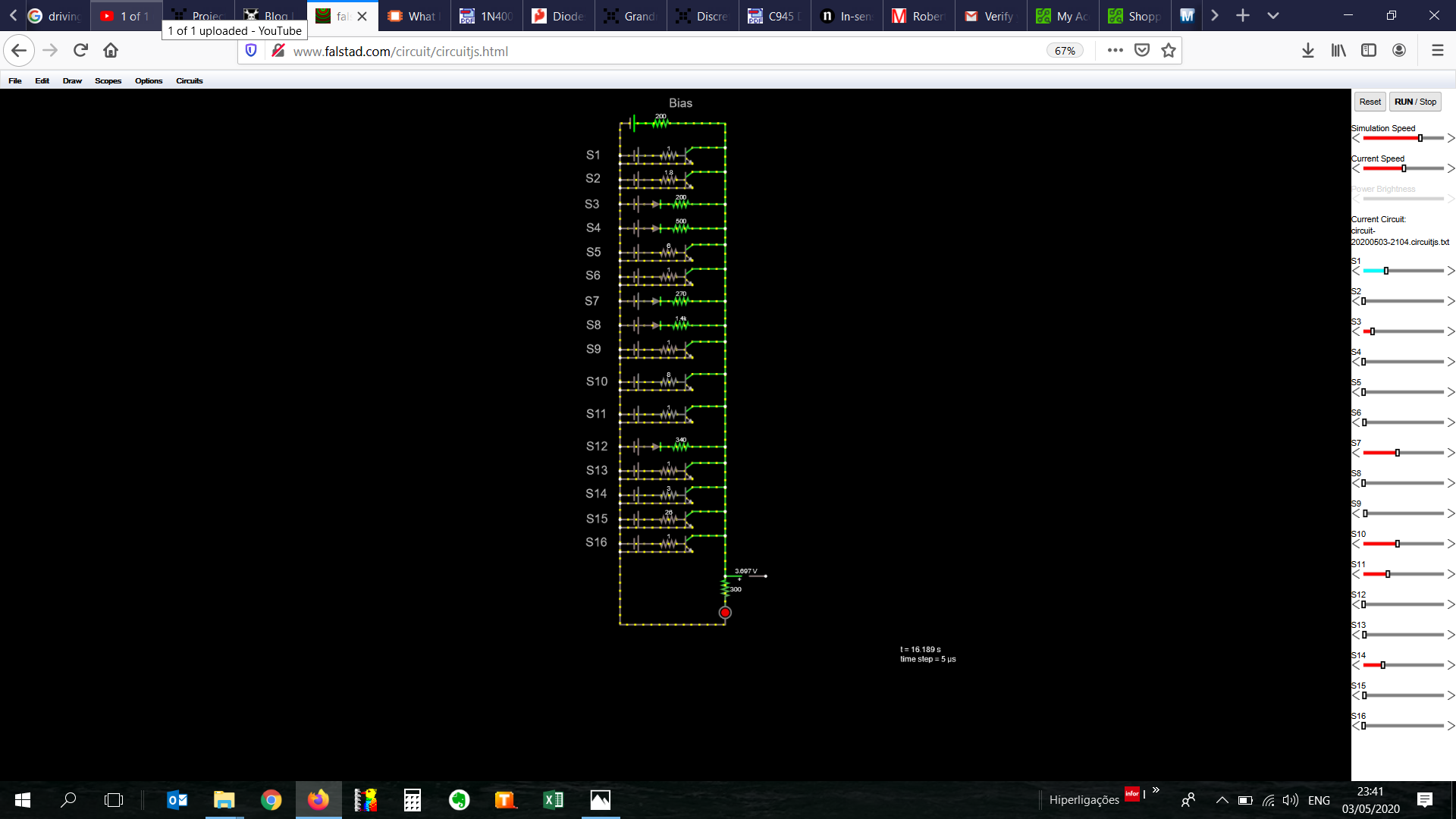
So, with my small simulation out of the way, I proceeded with a bigger simulation, with all 16-inputs weights punched into the circuit plus the bias. I then adjusted all the voltage values for a number which I knew that should light up the led and lo and behold, it worked!

What a freaking Eureka moment!

I had a working (virtual) circuit of a neural network. This was huge. Being able to translate a neural network model onto a functional circuit was really a very happy moment.

There were two important takeaways from this picture. The sliders on the right allow me to adjust the voltage of the input sensors. I then managed to see that adjusting the values of some of the sensors one way or the other, did not affect the result too much. The system is robust in a way that all 16 inputs have a say on what the number is, whereas in the decision tree, one sensor had the power to upend the whole thing.

So I had a working circuit, it was time to make a pcb.

Designing a PCB

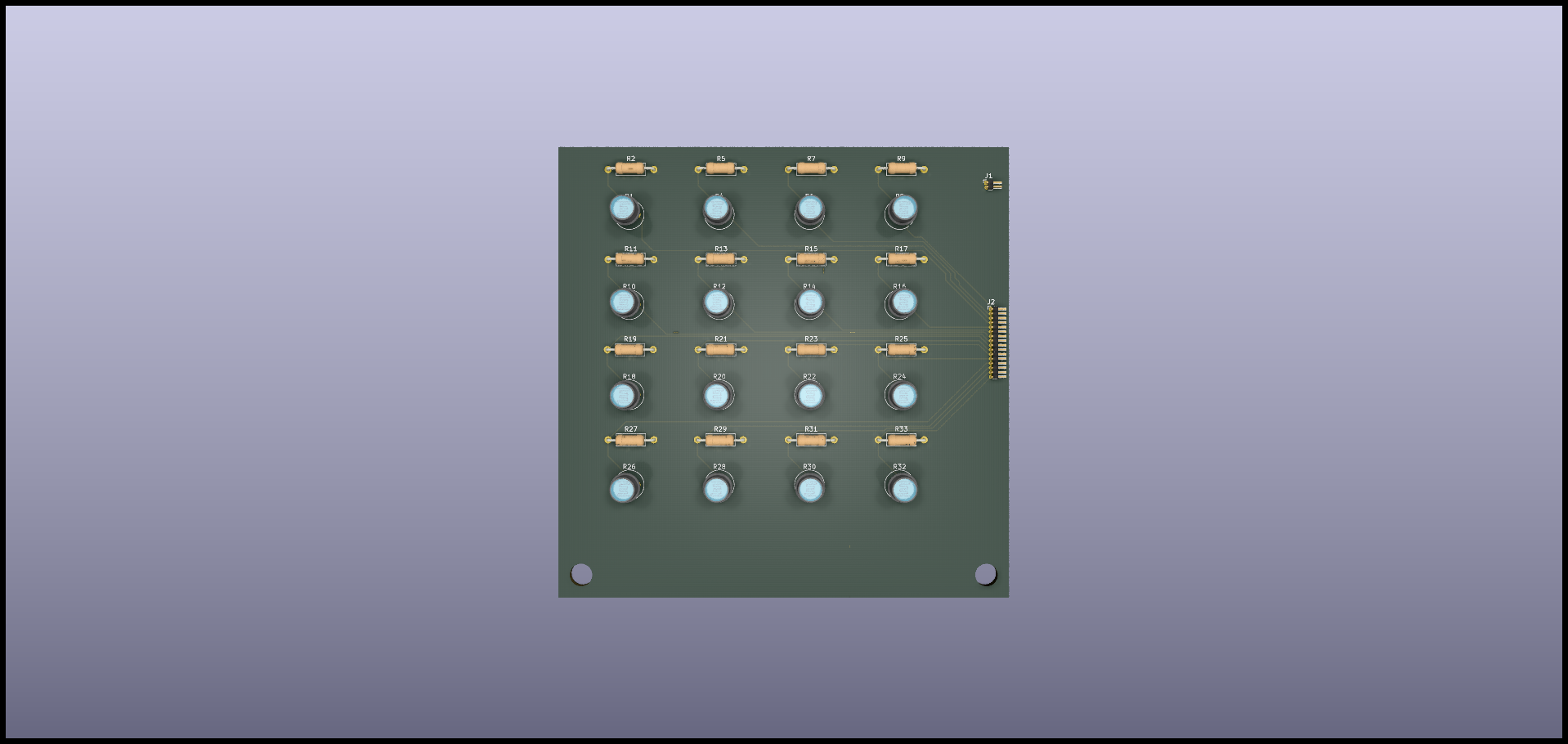
I never designed a PCB, but I thought I'd have a crack at it and started with the sensor matrix.

I read over an again people swearing by Eagle, then Kicad, then setting the comment section on fire, I decided in no particular order to try Eagle first. After a few tutorials and some messing around with schematics, I found myself severely limited with the free version of this software and moved on to Kicad. Honestly, it was not as painful as I was expecting the learning curve to be. I followed the video series from Ashley Mills and found myself making PCBs in no time.

The result was a square matrix of LDRs with their respective resistors to have the signal out already in the form of a divided voltage. The schematics and pcb file are attached here and here.

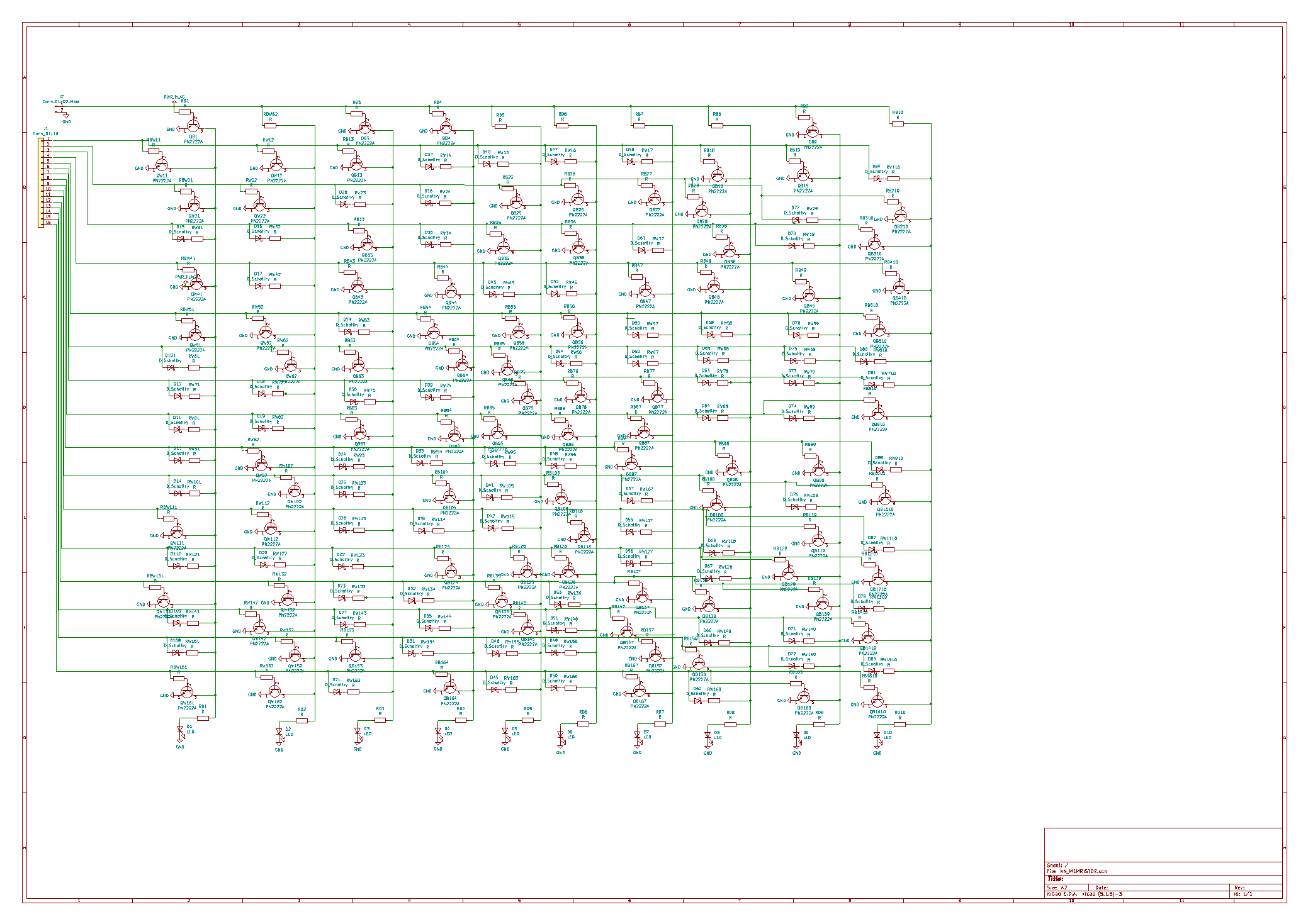
Since things were coming along nicely, I decided to have a go at designing a digit line for the memristor. After finishing the first line, I realised that the output didn't mean anything since the result is just the brightness of an LED. In order to tell apart whether it's a 1 or not, I'd have to have another LED saying which other number it could also be. So I decided to draw another digit line. In the end, I drew all 10 and realised the monstrosity this thing had become. The schematic fitted comfortably on an A2 piece of paper. This was bigger than I had bargained for. By far.

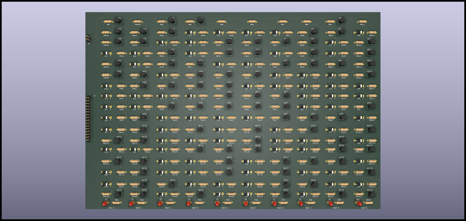
Eventually the schematic was placed on a board and could be fit onto an A4 size PCB. I'm pretty sure it can be made smaller, but then I'm also not very good at soldering so I tried to leave some space to work more comfortably. And I'm not sure I did a good job at that.

The resulting PCB looks like something I would have expected to see if I opened a machine some 30 years ago. The packed project can be found here.

Conclusion

It's a really exciting moment for the project and one I didn't think would come one day. The project was really focused on decision trees, not neural networks in mind. Nevertheless, things evolved naturally.

I did have a go at making a decision tree PCB, but then I dropped it very quickly to make the neural network.

It has been overall an incredibly fulfilling experience, and I have learnt a lot long the way.

Now the question is: Will it work? There's only one way to find out.

Disclaimer: I've never designed a PCB before and also don't have an EE background so use the information here contained with caution.

The goal of this task is to develop a solution to implement the neural network nodes using discrete components.

Initial idea

The initial idea was to use analog multipliers based on a SE discussion. The source also references an additional solution using a MOSFET, but I couldn't find a way to implement this. The other solutions were an AD633 analog multiplier and the MPY534, the latter a bit more expensive.

Either way, both solutions theoretically could work, nevertheless, it could get expensive quite fast. A quick back of an envelope calculation is, I'd need 10 nodes, with 16 multiplications and additions, then I'd end up needing 160 multipliers. The cheapest is the AD633, and it goes for around 10€ a piece. For 160, they come down to around 7€ each, or 420 € just on multipliers. That's a hard sell.

There was another solution mentioned using log-add-antilog OpAmp circuits. These would need also log amplifiers, and it becomes very expensive very quickly as well. In the end, the easiest to implement, and cheapest, was the analog multipliers.

All in all, this seems like a dead end, not even taking into account the fact that I have negative numbers to multiply. Maybe this is also possible with analog signals, but I cannot wrap my head around it.

I got it all wrong

It occurred to me that if this is so simple to implement, then someone must have done it before. So I started to do some research and got some papers from the 80s where people where designing VLSI chips to deal with neural networks. So, I cannot do VLSI, what else have you got?

More recently, the work from wolfgangouille stands out with the very cool implementation of neurons in his very cool Neurino project.

A bit more search got me to memristor bars from the nice video of Mr. Balasubramonian explaining his implementation. Now, memristor bars are really cool from the point of view of implementation, you've got voltage signals coming in, a bunch of resistors and conductors and finally a current output that should be transformed onto digital signal or voltage if needed. Hey, this is great!

Not so fast, we still have to deal with the negative values on the weights.

Some of the weighs that came with the model were negative. Now, memristors work by turning the input signal (a voltage) onto a current by passing through a resistor. The resulting current is the product of the voltage by the conductance of the resistor. So how on earth am I going to come up with a negative conductance resistor? Well, since I'm not EE trained, I didn't really know this was possible but Wikipedia proved me wrong.

Even though there are some conditions in which some semiconductors seem to show this behaviour, it didn't seem like an easy thing to throw in my NN. We needed a different solution.

Turning the problem upside down, I tried to reflect on what had to take place in my model circuit.

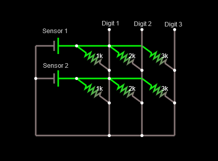
Case 1. Positive weight

In this case, the weight would be represented by a resistor, the voltage multiplied by the conductance would render a current. The current would be added to the current coming on the Digit 1 wire and would be transformed onto a signal at the exit.

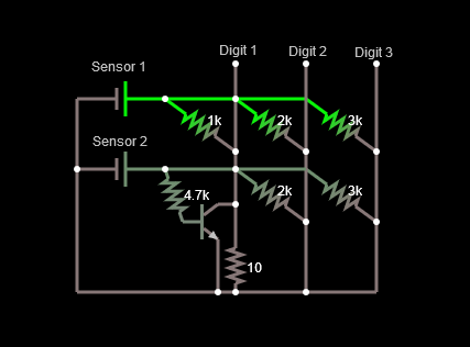
Case 2. Negative weight

In this case, instead of putting current into my wire, I'd need to substract the current from the wire. So, I just need to find a solution to remove current from the wire, right. Well, put like that it's more or less easy. The problem might be finding a linear way to do this, but a simple implementation can be found below. The negative weight is represented by a transistor driven by the current created by the voltage coming from the sensor and a resistor. As the transistor gets current across the base, it allows some of the current traveling through the wire to escape. Hence, the actual current in the Digit 1 ampmeter goes down as the voltage from the sensor increases.

Below is a short video of the memristor with the negative weight in action.

As the Sensor 1 voltage changes, all the outputs on Digits 1 to 3 increase as the currents are all produced with positive weigths.

As the voltage on Sensor 2 changes, the current signal for Digits 2 and 3 increases, whereas the current for Digit 1 decreases, reflecting a negative weight node.

The math need some attention since this is just a proof of concept. In order to get a proper signal treatment, proper choice of transistor and resistors will weigh on the accuracy of the results.

Signal constraints

We have solved the issues pertaining the design of the nodes of the neural network. Nonetheless, there is still another issue. The signal from the photoresistor is not linear as can be seen from the plot below.

There is two ways to work with LDRs as sensors. The first one is to work only in the linear regions, but then we'd need to make sure all the sensors have the same response which would allow a good quality signal. From my limited experience with LDRs, this can be tricky and I've found a lot of inconsistency in consecutive readouts. The second one is to work with binary signals, i.e. instead of reading out an intensity from the pixels, round the intensity values and read out 0s or 1s.

From the work carried out in the development of the decision trees, binary signals are much easier to read an manage when using LDRs. Nevertheless, a lot of information is lost and success using binary signals could be obtained only by using a bigger matrix.

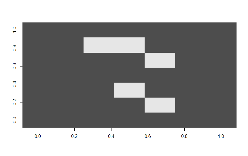
An example of a digit "5" with a binary 4x4 matrix versus a 7x7 matrix is depicted below. As can be seen, too much information is lost in the 4x4 matrix.

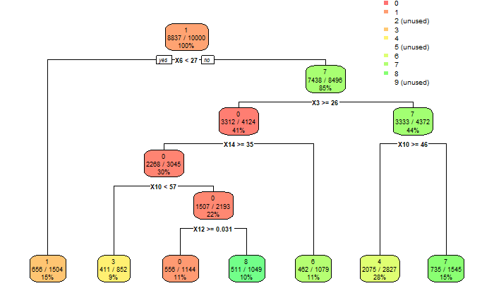
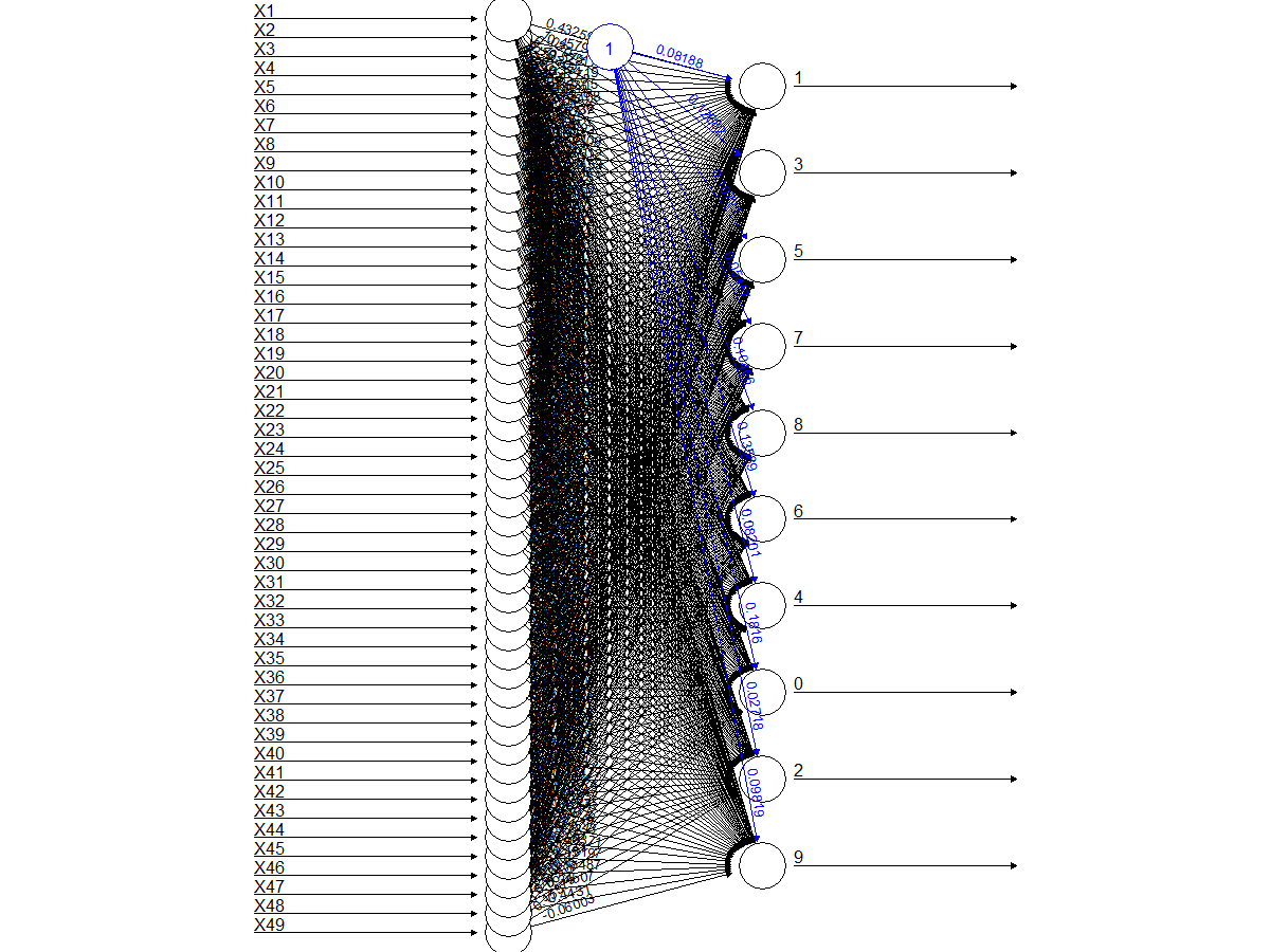
With a 7x7 binary matrix training a neural network using 1000 numbers, the model below is obtained with an acceptable accuracy.

The accuracy for each digit using the binary 7x7 matrix is as follows:

        0         1         2         3         4         5         6         7         8         9 
0.6105130 0.4642998 0.3916667 0.4367953 0.3751996 0.1865399 0.4743822 0.4334711 0.2476398 0.1370285 

Conclusion

A binary solution seems to be the best solution as long as we're keeping with the LDRs. Photo-diodes seem to be an alternative but I'm only getting comfortable to work with voltage signals for the time being.

Next, design my first PCB to detect MNIST digits using a neural network.

The goal of this task is to train the simplest neural network that could recognise digits from the MNIST database and make it compatible with a discrete component implementation.

Minimum Model Neural Network

This one is an easy one. The simplest neural network (NN) is one with just the inputs and the outputs, with no hidden layer.

This neural network has a total of 16 inputs which represent the pixels on the 4x4 matrix described in the Mimimum sensor log and 10 outputs representing the 10 digits or classes.

The confusion matrix for this model can be found below.

       0    1    2    3    4    5    6    7    8    9
  0  768   58   17   17    8    3   75    8  195   17
  1    0 1240    6   14   43   14    6   13    7   13
  2   26   91  708   61   57    0  171   28   63    5
  3   51  134  109  737   20   11   18  127   23   35
  4    4   94   13    0  592    6  112   95   27  191
  5  109   71    2   45  120  303  111   99  174   31
  6   42   45   44    0   95   11  945    2   26    2
  7    6   70    8   11   26    2    7  989    1  119
  8   45  189   19   34   16   20   61   30  656  102
  9   12  103   14    6  110    4   20  387   25  498

 The accuracy of the model was not bad, especially when compared with the decision tree or random forest models trained in the previous tasks.

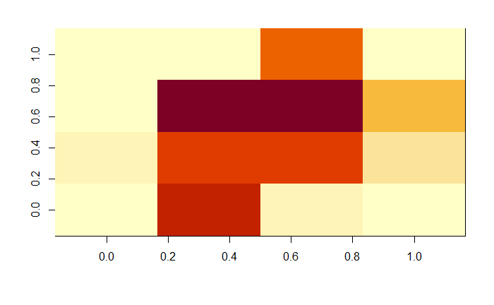
        0         1         2         3         4         5         6         7         8         9 
0.5256674 0.5608322 0.4909847 0.5072264 0.3634131 0.2667254 0.5270496 0.4876726 0.3829539 0.2939787

Some numbers don't fare well at all, but let us not forget this is a 4x4 matrix, even I couldn't tell the image below belonged to a 0.

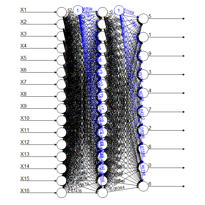
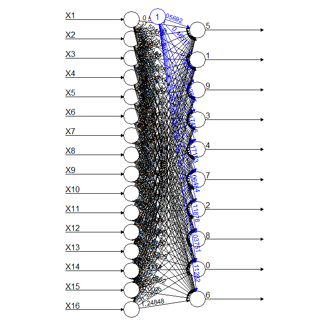
Of course a higher pixel density will improve the accuracy of the model but I'm more interested for the time being in simplicity at the expense of accuracy.

So this was the simplest NN model I could come up with, so we introduced some complexity to see how much we could improve the accuracy. The first model had a single hidden layer with 16 nodes as shown below together with the accuracy values for each digit.

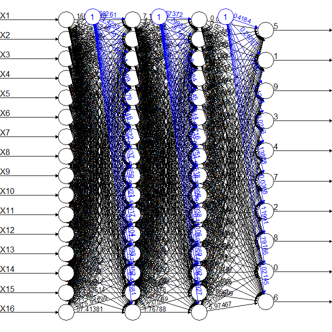
        0         1         2         3         4         5         6         7         8         9 
0.5044997 0.6573107 0.5772171 0.5874499 0.4180602 0.5212766 0.6659436 0.4793213 0.4176594 0.3957754 

The accuracy increased in some digits, but not so much as to justify the increase in complexity. The second model had two hidden layers with 16 nodes each, as shown below together with the accuracy values.

        0         1         2         3         4         5         6         7         8         9 
0.4885246 0.7461996 0.5099656 0.4409938 0.4449908 0.4448424 0.6528804 0.5533742 0.3882195 0.2722791 

The accuracy of the second model with two hidden layers was better than with one layer, but not for all digits and the cost is realy high in terms of complexity. Overall, the best trade off between complexity and accuracy was the first model.

Breaking down the maths

As neural networks go, they're as simple as they come. The nodes receive the inputs, multiply them by a weight and add a bias. Piece of cake.

The result is then for each node:

That means that knowing the weights and bias of an output node we could in principle calculate its probability with very simple maths.

For example, for the first model shown at the top of the page, the weights for each sensor and the bias for the output node for digit "5" are:

       Input      Weight       Signal       Product
1       Bias -0.05691852          N/A   -0.05691852
2   Sensor 1   0.5397329            0             0
3   Sensor 2  -0.4359923  0.004321729   -0.00188424
4   Sensor 3   0.3074641    0.2772309    0.08523854
5   Sensor 4  -0.4892472 0.0004801921 -0.0002349326
6   Sensor 5  -0.5862908            0             0
7   Sensor 6    0.231549    0.4101641    0.09497309
8   Sensor 7  -0.0697618    0.4403361   -0.03071864
9   Sensor 8   0.5010364     0.164946    0.08264393
10  Sensor 9    1.150069   0.04017607    0.04620524
11 Sensor 10   0.1367729    0.3277311    0.04482472
12 Sensor 11  -0.3862879    0.3078832    -0.1189315
13 Sensor 12   0.7872604   0.08947579    0.07044075
14 Sensor 13   -0.273486  0.009043617  -0.002473303
15 Sensor 14   0.3749847    0.3589436     0.1345983
16 Sensor 15   0.5307104   0.05786315    0.03070857
17 Sensor 16  -0.8331957            0             0
                          Total:         0.378472

 Multiplying the response array from the sensor and adding the bias I can get the result for digit 5, in this case, 0.378472.

Easy, so now we need to implement this using discrete components.

The goal of this task is to look into the future and determine other potential ML algorithms that could be implemented using discrete components.

Cats vs Dogs

MNIST digit recognition was nice to start with, but it's kind of the "hello world" of object recognition. Hence in the last log I focused a little bit on what could be an interesting challenge as a goal to bring Discrete component object recognition to the masses.

An appealing idea was to get the discrete components to tell apart cats versus dogs. That would have been perfect, so I set sail to try and have a decision tree tell apart cats and dogs.

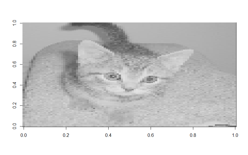
The dataset was the cats vs dogs dataset from Kaggle, imported into R using the imageR package to crop the pictures square, resize them all to 100x100 pixels and reduce the RGB channels to a single grayscale intensity scale.

The images were nowhere near as pretty as the original, but I could tell apart a cat from a dog without much effort, so I expected the algorithms to do the same.

The decision tree was trained using the rpart R package and the accuracy was calculated using the same metrics used in the previous logs. In short, the number of identified cats was divided by the total of (identified cats + false cats + false dogs).

The accuracy results were short of appalling, no matter how complex the decision tree was made or how large the training set used.

 Confusion matrix
     cat  dog
cat 1034  566
dog  827  773

Accuracy
      Cats       Dogs 
 0.4260404  0.3568790 

So after looking at the pictures for a while I realised that DT were never really going to cut this, no matter how complex they were since the cats were always in different places in the image, with many other artifacts appearing around them. So I thought, this called for random forests (RF).

RF should address all of my issues, they'd build trees in different places around the image and get a better weighted response. Nevertheless, if this was indeed to be a Discrete Component affair, then I had to try and limit the size of the model. The R caret package has a standard random forest size of 500 individual trees. There is no way that is going to be built no matter how many years I had to stay at home. So I tried first with 10 trees, then 20, then 50, then 100 and then I realised this was also not going to fly.

The accuracy was indeed better, but not really the improvement I was expecting.

 Confusion matrix     
     cat  dog
cat 1043  557
dog  652  948

Accuracy      
     Cats        Dogs  
0.4631439   0.4394993

At this point I started to read about tree depth, impact of number of trees and realised that I needed a lot more trees and nodes to make this work. Cats and dogs was not going to be easy.

Nevertheless it gave me an idea. What if I could implement more trees in the MNIST model, whilst keeping the number of nodes reasonably low?

MNIST was not so boring after all

So I came back to the MNIST dataset and tried to test the null hypothesis:

"For the same overall number of nodes, decision trees have the same accuracy as random forest models"

I started with a random forest with a single decision tree, maximum 20 nodes. The accuracy results were:

        0         1         2         3         4         5         6         7         8         9 
0.4165733 0.5352261 0.3046776 0.2667543 0.3531469 0.0000000 0.2709812 0.3712766 0.1717026 0.2116372 

Not pretty, but in line with I had already obtained in the minimum model using 10000 records.

So, with the benchmark set, I trained a random forest with two decision trees, maximum 10 nodes each. And the results were:

        0         1         2         3         4         5         6         7         8         9 
0.4800394 0.2957070 0.2172073 0.2161445 0.2116564 0.1522659 0.1727875 0.1840206 0.1464000 0.1265281 

Surprise! For most digits, the random forest fared much worst than the single tree. There goes my null hypothesis.

I wouldn't give up so easily so I increased the number of nodes and trees with more or less the same results.

Only once I really increased the number of nodes to 1000 did I notice a difference between the two algorithms. For a single 1000-node tree the accuracy was:

        0         1         2         3         4         5         6         7         8         9 
0.6784969 0.7598280 0.5159106 0.4412485 0.4515939 0.4144869 0.6269678 0.5813234 0.3870130 0.4326037 

For a random forest of 20 trees with maximum 50 nodes each, total 1000 nodes as in the above model, the accuracy was:

        0         1         2         3         4         5         6         7         8         9 
0.8503351 0.7897623 0.6440799 0.5855583 0.6387727 0.4900605 0.7507225 0.6986129 0.5977742 0.5315034 

This is a significant improvement for all the digits, but at this complexity level, it's kind of difficult to build a discrete component system.

An interesting idea was, maybe the fact that we have a lot of trees helps. What would happen if I use 50 trees with 20 nodes max each, I'd still use 1000 nodes total? The answer was kind of disappointing. The accuracy was actually worse than having 20 trees and 50 nodes, but still better than the single tree.

In the end, the null hypothesis was destroyed. Twice.

For a small number of nodes, decision trees are better than random forests. For a lot of nodes, random forests trump decision trees.

Schroedinger's cats and dogs

I was also very disappointed when I came to the realisation that at least half of the cats and dogs in these pictures were dead. The kaggle dataset was 6 years old. I'd safely assume the pictures to be at least as old as the dataset and considering the life expectancy of cats and dogs, we're well past the half life of the dataset.

The future

Well, I was wondering, random forests are a no go. Decision trees don't really cut it. Why not neural networks (NN)?

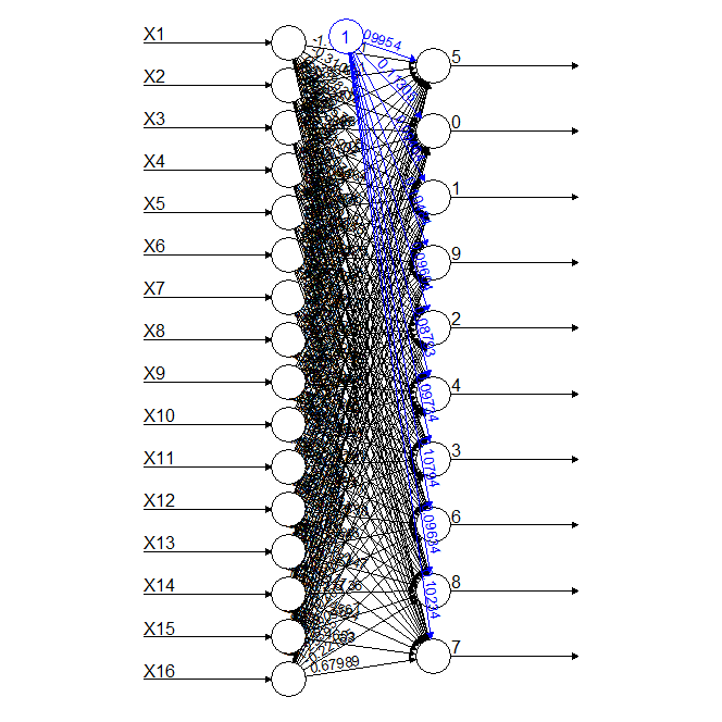
As far as I could remember NNs tend to have multiplication and additions, that's all. Could this be implemented using discrete components? Below is an example of a NN accepting all 16-pixels from the 4x4 MNIST digital matrix.

So, let's assume we have the signals from the pixel sensors (LDRs). The signal would have been a 1 or a 0, or a higher voltage versus a lower voltage. Could I multiply this voltage by a constant (voltage) and add it to another voltage multiplied by a different constant (voltage)? This was a humbling moment for me since I realised how little I knew about the treatment of analog signals in general.

So, for those of you who also don't have an EE background, you can add voltages, and you can multiply them as well, all using discrete components.

We'd need a summing amplifier and an analog multiplier. So these are quite common components (still quite discrete if you ask me) and even some of the analog multipliers accept an offset, i.e. I could multiply and add in the same component.

I've just found myself the building blocks for a discrete component neural network.

This project is just getting started,

The goal of this task is to actually make the digital implementation work.

Forget Mr. Fields

So, I had a go at the why the previous circuit was not working, and I found out it was just messed up in so many dimensions it's hard to name them.

In the end, I spent a lot of time learning, which I think that's what projects are for. I've got a much better grasp about the behaviour of NPN transistors and RTL, previously all dark arts for me.

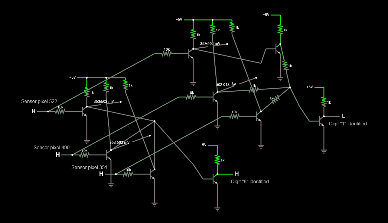
The circuit below describes the actual implementation of the left arm of the above decision tree implemented with RTL. I couldn't attach the circuit file, something wrong with the HAD.io platform today.

So, implementation via RTL is possible, but a PIA, even for simple trees. Even locked up at home with nothing better to do.

A much better solution would be to implement this via e.g. 74AS logic gate circuits. These have a theoretical propagation time of 2ns for the faster chips. The most complex decision tree discussed in the Bonus Track log, was 11 levels deep. That means that adding up the times of all the gates, the response time would be of 22 ns, or a detection frequency of 40 MHz. This does not tell the whole story since half of these would have to carry inverters on the way, but still, not very far off from these numbers. Not bad for a bunch of transistors.

Conclusion

Finally we have reached the point where we have managed to implement both analog and digital solutions to the Discrete Component Object Recognition System.

From an implementation point of view, the digital solution is the most robust, the fastest one and the one least likely to cause headaches. It's also the most forgiving in terms of sensors since it can readily work with LDRs, despite their relatively slow response time.

Future work

Well, wouldn't it be nice if more complex images could be recognized instead of just the MNIST numbers? What about cats and dogs?

The goal of this task is to make a prototype of the digital version of the discrete component object recognition system.

Digital implementation

Once it was clear that there was a digital pathway, I set forth to building a prototype.

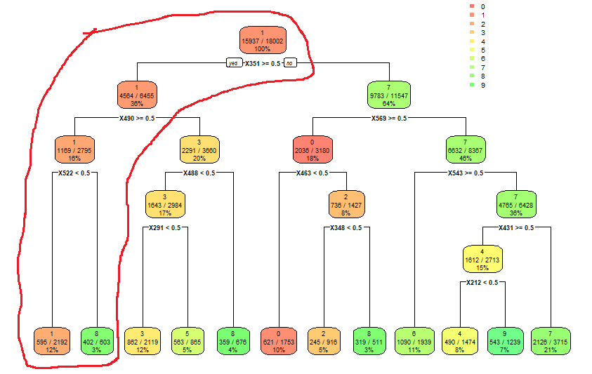
The first prototype was based on the leftmost pathway of the decision tree below.

This would allow us to identify 100% of the "1" with an accuracy of 53% and about 30% of the "8" with an accuracy of 20%. This accuracy of 20% doesn't sound like much but let's not forget that a monkey pulling bananas hanging on strings would get 10% and this is a proof of concept. We can increase the accuracy, but I'd need a lot more sensors, and probably a more robust setup than dangly Aliexpress breadboards.

By the way, does anyone know of a trick to secure resistors in place on a breadboard? The connection is sketchy and drives me mad.

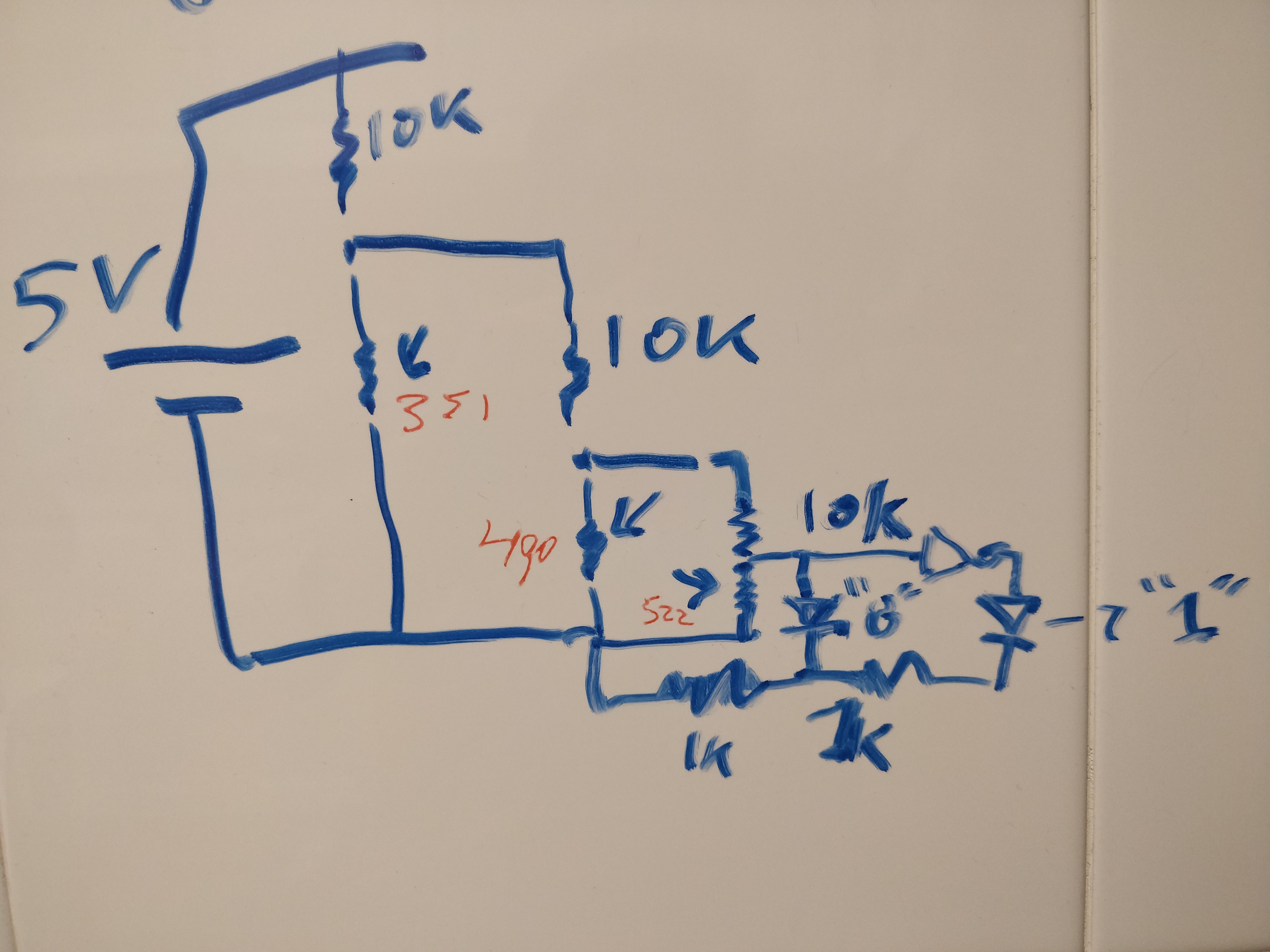
So, I sketched the circuit on kicad on the kitchen tiles and got to build onto a breadboard.

Later on I realized that there was a small mistake on my drawing but this got quickly corrected on the breadboard.

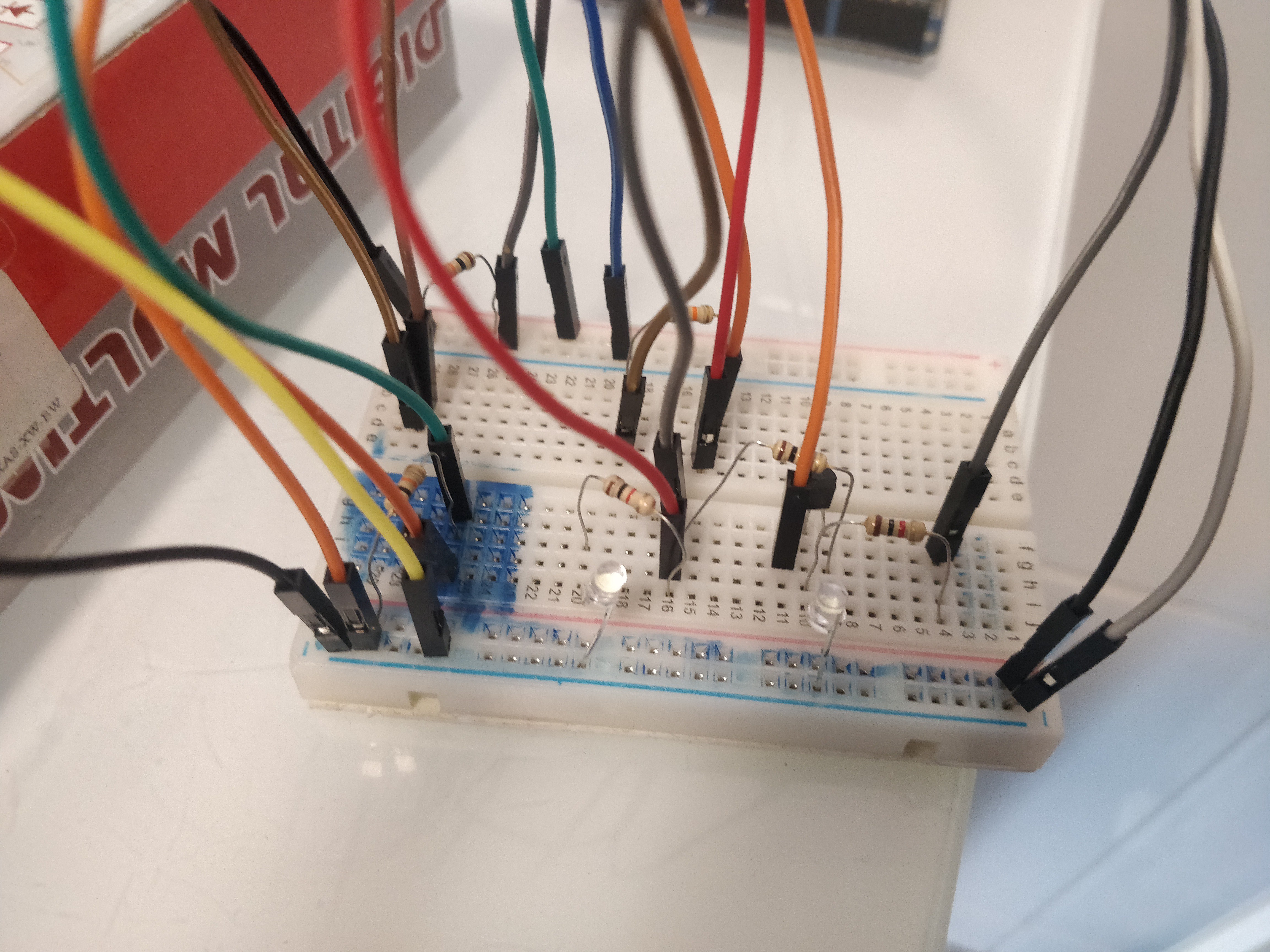
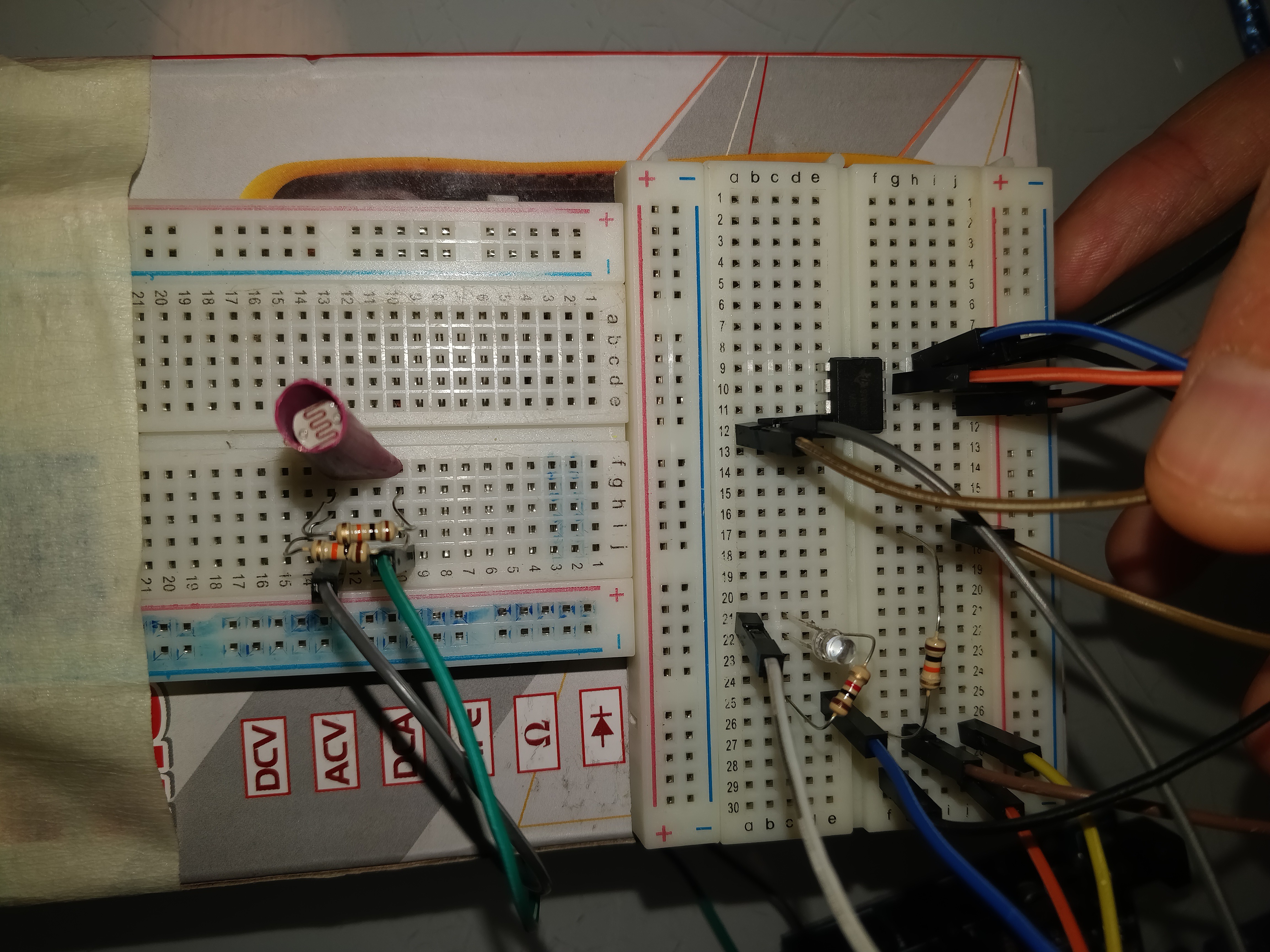
Below is a picture of half the setup, not including the sensors. This is probably not what comes to your mind when someone asks you to picture Artificial Intelligence.

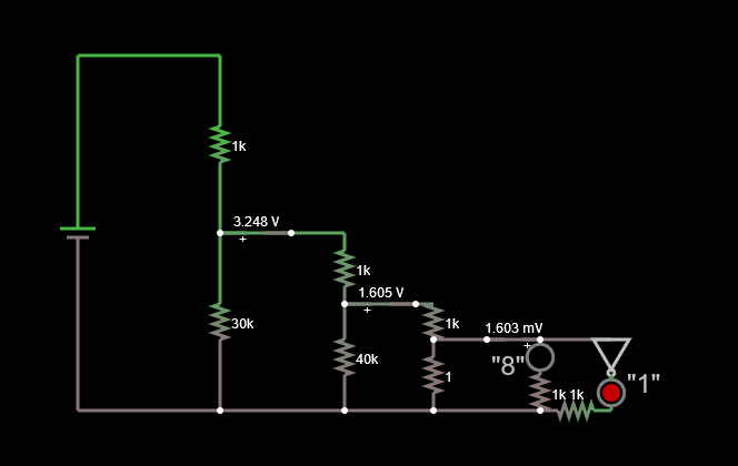
In the end, as usual, the circuit didn't work. I used the Falstad circuit simulation tool to see what was going on and found out that the voltage I was using was too low to drive the LEDs at the other end if the circuit.

There was not enough voltage to even get a signal and read from the Arduino so it was easier to play with the values on the DC source until a reasonable signal would come out of the other end. In the end, it was a 12V DC source that did it.

Even spending a few hours changing resistor values and rerouting signals did not get me any closer to using both LEDs successfully, After a bit of thinking about the circuit, I realized that once one resistor upstream changed so did the other voltages downstream, so nothing was completely black and white after all. I really need some help to figure out how to implement the circuit for this system.

In the end, I couldn't let my lack of know-how on testing the feasibility of the concept, so I resorted to my good old trusty Arduino to do the ADC for me and let me know whether a 1 or an 8 was being identified.

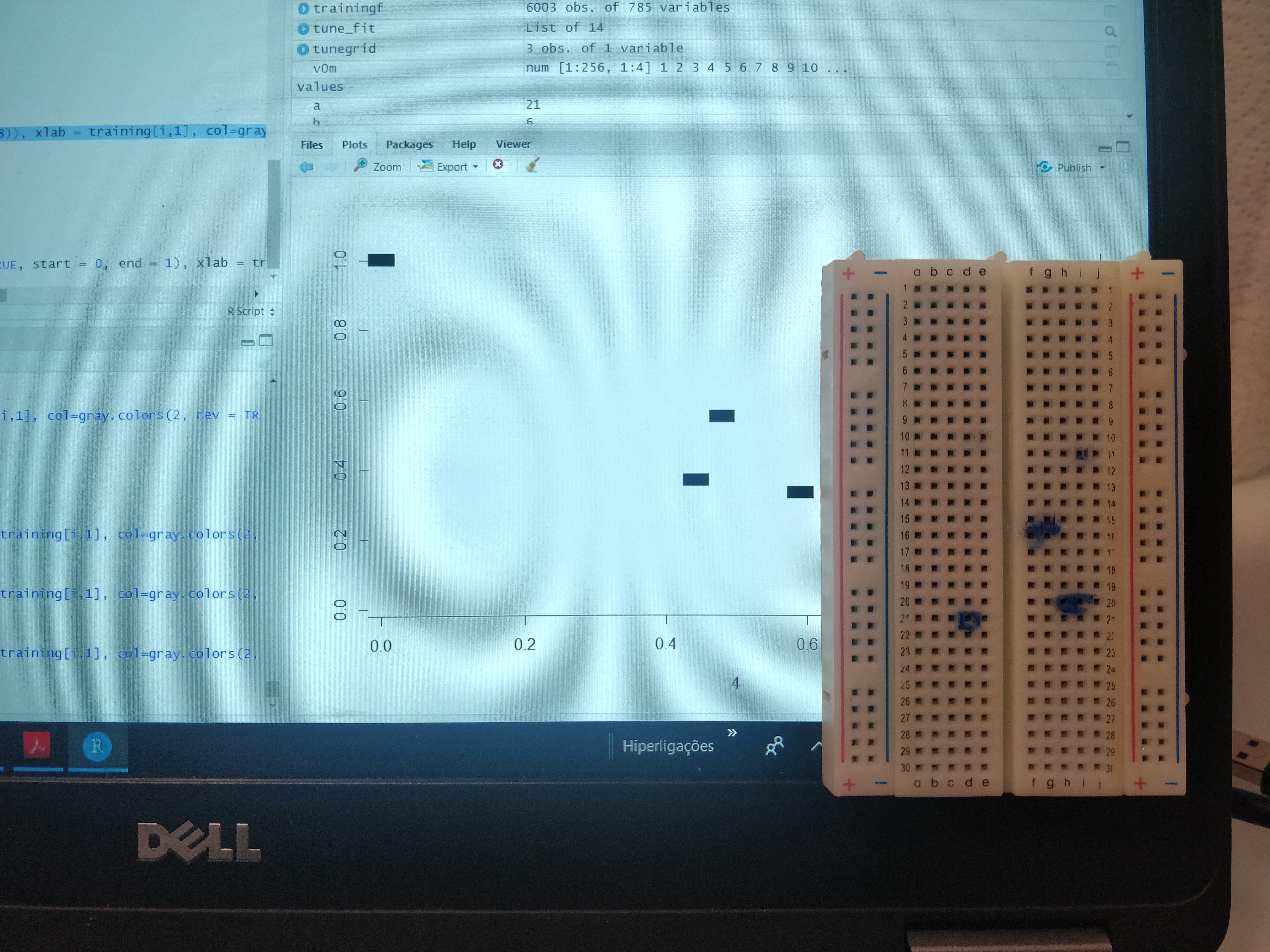
For the sensing side, The relevant pixels were drawn on the screen in order to setup the alignment on the breadboard and mount the sensors.

Once the sensors were mounted, the alignment was verified and the setup was ready for testing.

Test drive

For the tests, the same MO was used as in the previous tasks, i.e. cycling digits on the screen, reading the voltage via the ADC on the Arduino UNO, print()ing the values to serial and reading the serial from Rstudio where it would get compared to the number displayed. The information would then be recorded on a confusion matrix.

All went well with the Arduino, the ADC behaved beautifully and the signals for the binary 0 and 1 were clearly distinguishable from the voltage readings. Nevertheless, once I started testing, I realized that my sensors were too big for the pixels.

Too big sensors? No problem I thought, we just increase the pixel size. The matrix was averaged to reduce the pixel size by half but since numbers tend to be thin by nature, then a lot of traces got erased during the translation from gray scale to black and white. This meant that even I could not tell the numbers apart.

As W.C. Fields said:

If at first you don't succeed, try, try again. Then quit. No use being a damn fool about it.

Conclusion

It's probably possible to make a binary system work, but with my current limitations I could only continue with some help on getting the circuit to do my bidding, and smaller sensors to measure said pixels.

I'll try to find a way to make the sensors smaller, or get smaller sensors. To be continued.

Whilst thinking about the results obtained and licking my LDR inflicted wounds, I thought about a way to implement this object recognition system that would not involve fiddly hard to measure intensity levels.

It occurred to me that I could change the intensity levels from 256 shades of grey, to a binary 0/1, i.e. if the intensity was higher than 127, then 1, else 0. In this way, the pictures become black and white, instead of grey shades, and we have new implementation possibilities.

Up til now we needed to measure an intensity, translate it onto an analog signal (voltage), compare it to the reference voltage and get a digital signal (In each split node: Yes/No, Left/Right, etc).

Now, we have a binary signal, we do not need to fiddle with intensity levels, analog signals, we do not need voltage comparators.

Heaven.

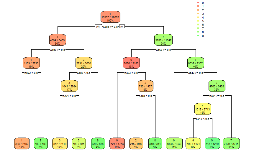
Below is a decision tree modeled on the same MNIST dataset but using the new binary system instead of the intensity level. The accuracy is in line with the models obtained in the Minimum Model task using all the default settings in Rstudio and the rpart package.

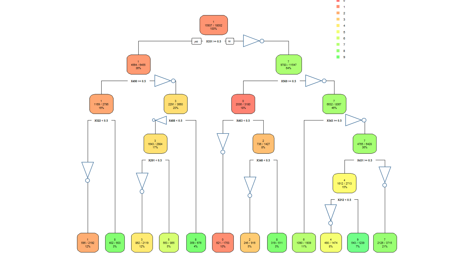
The confusion matrix below shows that a lot of digits get miss-classified. Nevertheless, this model has not been optimized nor iterated in any way. The columns represent the digit shown and the rows represent how they were classified.

       0    1    2    3    4    5    6    7    8    9
  0  757    4    1   28    6   51  149  131   32   23
  1    6 1036   17  151    0    7   18   67   55    1
  2  120   78  458   26   39    2  168  110  169   22
  3   43   23   14  864   24   65    5  129   47   31
  4    3   27    5   31  665   28   64  220   23   88
  5  118   30   20  166   72  211   35  215   88  128
  6   67   35   50   24  102   19  585   61  268   24
  7    4   28   10   21   31   57   42  961   13   31
  8   36  143   51   68   19   34  205  146  391   40
  9    5   40    2   64   91  154   51  330   19  462

 The overall accuracy was just over 53% and the individual accuracy is shown in the table below.

        0         1         2         3         4         5         6         7         8         9 
0.4779040 0.5866365 0.3362702 0.4736842 0.4323797 0.1406667 0.2966531 0.3686229 0.2116946 0.2876712 

There is a huge improvement potential with this change.

• There is no need to calibrate the LDRs, the change in resistance between the 0 and 1 is enough to give a binary output
• There is no need to use voltage comparators, now transistors is all that is needed, implemented as NOT gates.

1. 11 LDRs
2. 11 NOT gates (can be built using 1 transistor and 2 resistors per gate)

Adding complexity

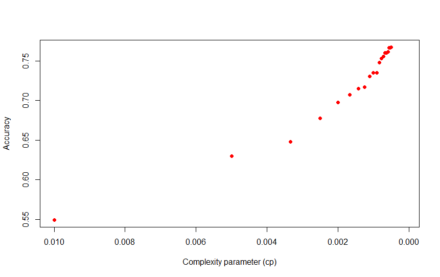
By changing the complexity parameter (cp), we can increase the accuracy significantly, at model complexity cost. The plot below shows the increase in accuracy as we reduce the cp value.

As cp decreases so does the number of splits. A model with a cp of 0.005 for example, has a sizeable jump in accuracy to 62 %, with a still manageable 24-node tree.

A step up to 0.001, increases accuracy to a respectable 74 %, with a 91-node decision tree.

There's a clear trade-off between complexity and accuracy, though more specific optimizations could potentially be carried out in order to obtain a better accuracy without a high complexity penalty.

Conclusion

We have reached a solution that could allow us to implement a really simple object recognition system using readily available components.

The accuracy could be considered to be within the goals of the project at a respectable 75 % plus if we're willing to live with the complexity level.

As a proof of concept this project allows for potential improvements by using more complex decision trees and replacing more elaborate, slower and less power efficient systems in Object Recognition applications.

The goal of this task was to validate the concept using discrete components, the reduced decision tree obtained in the Minimum hardware task and measure its accuracy.

The model

The model to be used was the one below, discussed and analyzed in a previous task.

The hardware

Due to stock and time limitations, only one LM393P voltage comparator was available, hence two splits could be implemented. The prototype was only going to be able to detect "Number 1" or "Numbers 4 or 7" by analyzing the signal from pixels 6 and 3. Nevertheless, only one of the LDRs used throughout this project was actually able to measure with acceptable drift and jitter so only digit "1" from the MNIST database was detected.

Since we had a single digit to identify, a single LED was used to inform whether the digit being shown had been identified as a "1". In order to build the confusion matrix, the LED voltage was recorded by the Arduino UNO.

The video below shows the setup in action.

The confusion matrix is attached below.

        [,1] [,2] [,3] [,4] [,5] [,6] [,7] [,8] [,9] [,10]
 [1,]     18   11    4    2    3    1    2    0    1     0
 [Not 1,]  9   11   16   22   15   19   16   15   22     0

The accuracy towards number 1 was 35.2%. This was below the performance obtained with the micro-controller which is disappointing. I really wanted to get a better value using only discrete components.

Below is a close-up of the setup including the lonely LM393 in the center of the control breadboard and the single LDR on the "camera" breadboard. Since the screen brightness did not match the activation level for the voltage comparator, two 1k.ohm resistors were used in parallel with the LDR to align the sensitivity of the sensor to the screen intensity.

The final fine-tuning was carried out by displaying the target intensity on the screen and adjusting the screen brightness until the LED would be triggered around the level defined by the decision tree.

Speed test

In order to see how fast the system could detect the numbers, the numbers were drawn at increasing speed until the system could not catch up.

The test started at 1 Hz, was then increase to 10 Hz, then 20 Hz and 50 Hz.

The surprising result was that the system could keep up, but the screen could not.

In the video below, we can see the system recognizing number 1 at 20 Hz.

Nevertheless, the system could not be run any faster than this speed. The reason for this is that the screen could not draw the digits at the 50 Hz target speed.

Future work

Stock MNIST performance

The project was carried out using an averaged version of the MNIST dataset wherein the matrix was reduced to a 4x4 matrix from the original 28x28. The question that remains is, what would be the accuracy of the system when using the original database.

Implementing a more robust decision tree

This project proved that it's possible to implement a simple object recognition system using decision trees and discrete components. Nevertheless, a single split hardly represents a decision tree. A more complex decision tree would have been nice to test, given more time and the availability of parts.

Using the right tools

LDRs are definitely not to be used for these kind of projects. Maybe you can make them work, but the ones I had showed to be pretty unreliable.

A more robust system could probably be built with better sensors given the time. As Starhawk suggested, maybe photodiodes could be used instead with better results.

More voltage comparators for a larger tree would mean also that we'd need plenty of individual discrete voltage values. In order to have those delivered to the right comparators, a lot of voltage dividers could be used, but it could get complex pretty quickly. I wonder whether there are better tools.

Measuring the speed

Well, speed was one of the main drivers of this system and checking how fast it could go one of the objectives. Nevertheless, the screen refresh rate was the limiting factor in speed measurement.

From my point of view, the speed would be limited by the speed of the LDRs, with a response time in the order of 10 to 100 ms. Photodiodes on the other hand have response times starting at 20 ns, another reason to switch.

Either way, having a screen show the images faster than 100 Hz would be quite difficult. Any ideas of how to test this, if it does make any sense at all to test it, would be welcome.

Conclusion

We eventually managed to have a discrete component object recognition system.

It wasn't fancy.

It couldn't recognize a lot of numbers.

It couldn't even recognize the only number it was programmed to well.

All in all, it didn't fare great, the accuracy was rather poor.

Considering the goals of the project:

• Only discrete pixel sensors, CHECK
• Decision tree recognition, CHECK
• No microcontroller, PC or FPGA, CHECK
• 75% accuracy, not really, by a long shot

We can agree to a partial success.

All in all, it was quite a learning experience and extremely satisfying to see a simple LDR aided by a few resistors and a voltage comparator do the work we normally assume microcontrollers can do.

The goal of this task is to prototype the solution using a micro-controller to validate the concept

The Arduino prototype

An Arduino Uno did not really match the minimum hardware philosophy, but I had nothing less fancy to try it on. And the focus was on making sure it worked on the micro-controller in order to move on to the next task.

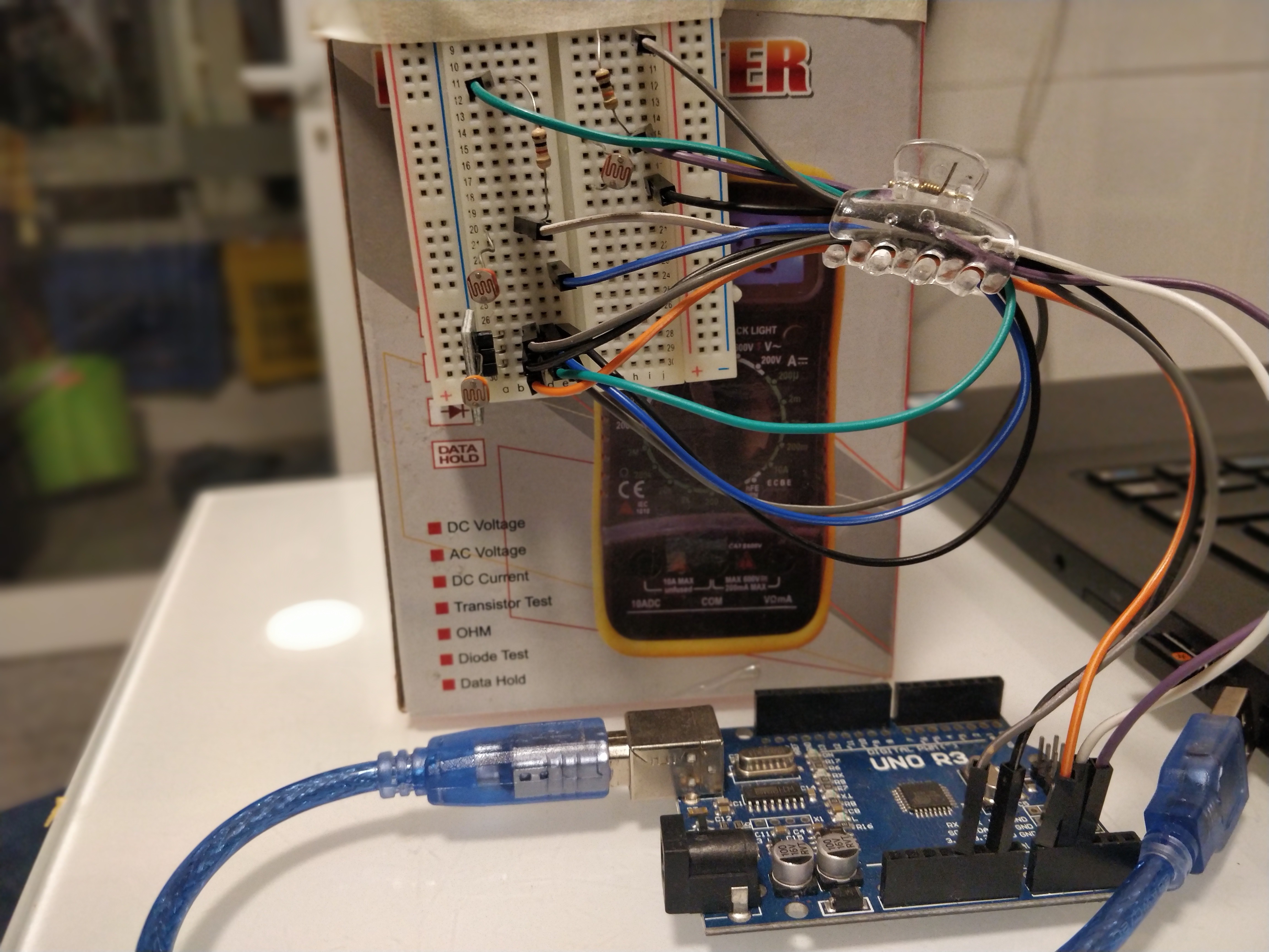
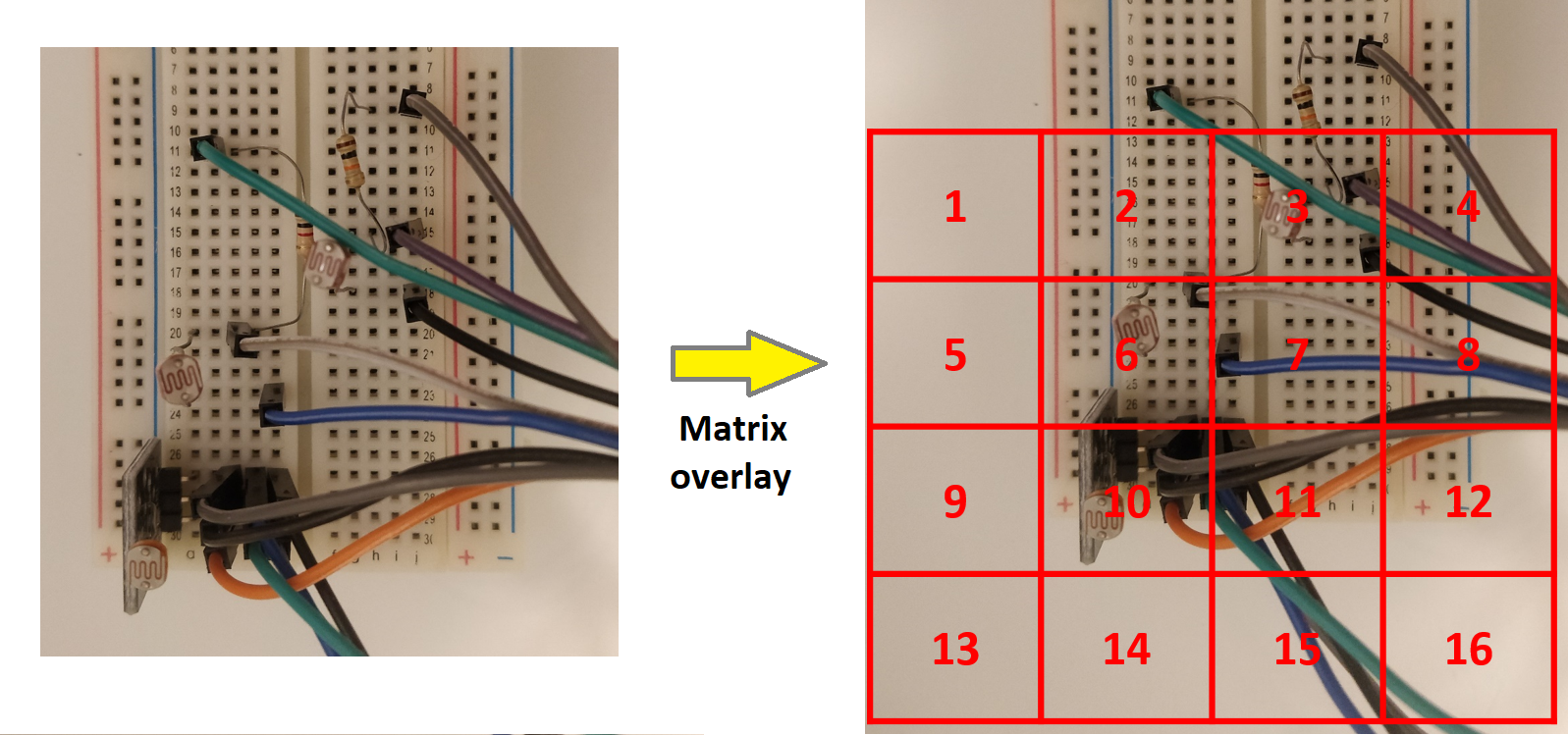
The prototype was set up to detect 3 digits from the minimum sensor model below.

The digits to be detected were "1", "4" and "7", using a total of 3 LDR sensors for pixels 3, 6 and 10.

The set-up worked as follows:

• Each LDR was a part of a voltage divider with a 10 k.ohm resistor.
• The LDRs were of 14 k.ohm (pixel 10), 40 k.ohm (pixel 6) and 60 k.ohm (pixel 3).
• The sensors were aligned with the matrix on the screen in order to capture the the analog output on each pixel.
• The matrix representing the number was drawn on the screen of a laptop using Rstudio.
• The response of the LDRs was calibrated using an intensity sweep before each test.
• The resulting voltage was read via the ADC on the Arduino on pins A0, A1 and A2 and 3 simple if-then loops represented the splits on the Decision tree.
• Both voltage and likelihood of a number being identified was print()ed to the serial monitor.

The matrix was drawn on the screen and cycled trough the dataset.

Finally, the jig was placed in front of the screen. Both displayed digit and detected digit were recorded and filled a confusion matrix to verify the accuracy of the setup.

In the end, the setup worked as expected, with the numbers 1, 4 and 7 being identified, sometimes.The accuracy, nevertheless, was appalling.

All in all, it was mighty difficult to get a consistent reading out of anything other than digit "1". And of course that depends on your definition of consistent.

Below is the confusion matrix for the prototype. Columns denote the number shown, rows the number identified by the decision tree. Note that if it was not a 1, 4 or 7, the model was set up to classify everything else as a 0.

      [,1] [,2] [,3] [,4] [,5] [,6] [,7] [,8] [,9]  [,0]
 [1,]   15    1    5    6    1    2    3    0    4     0
 [2,]    0    0    0    0    0    0    0    0    0     0
 [3,]    0    0    0    0    0    0    0    0    0     0
 [4,]    5    1    1    3    5    0    6    0    5     0
 [5,]    0    0    0    0    0    0    0    0    0     0
 [6,]    0    0    0    0    0    0    0    0    0     0
 [7,]    3    9    1    7    2    8    0    6    3     0
 [8,]    0    0    0    0    0    0    0    0    0     0
 [9,]    0    0    0    0    0    0    0    0    0     0
 [0,]    0    0    0    2    2    0    2    0    4     0

 The accuracy of digit 1 is just over 33%. For number 4, it's 7 % and for number 7, well, not a single 7 was identified correctly.

It was well short of the accuracy I was expecting to obtain with the setup so a bit of troubleshooting was in order.

Debugging

Cross-talk

In order to verify whether there was any issues with the intensity of neighboring cells on the matrix affecting the reading of the sensors, the setup was modified using a molding balloon cut to length in order to shield the sensors from light coming from the sides.

The resulting setup with the protected sensors is shown below.

There was no significant difference in the overall accuracy, so this was not really what was causing havoc in the system.

Sensor accuracy

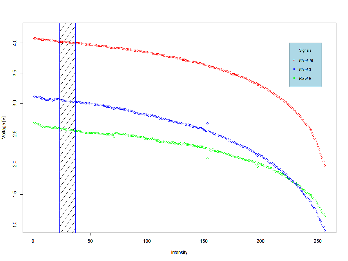
The decision tree splits happened at very low intensity values for these sensors, i.e. the sensors needed to measure values very close to the edge of their envelopes. The plot below shows the voltage versus intensity for all three sensors and the area where they'd be causing a split on the decision tree.

Even though the sensors are close the the edge of the envelope, there's plenty of measurement real estate available. This was probably not the cause for the accuracy issue but the plot shows that there was some jitter in the signal which is shown as deviations in the measurements, but only in some sensors.

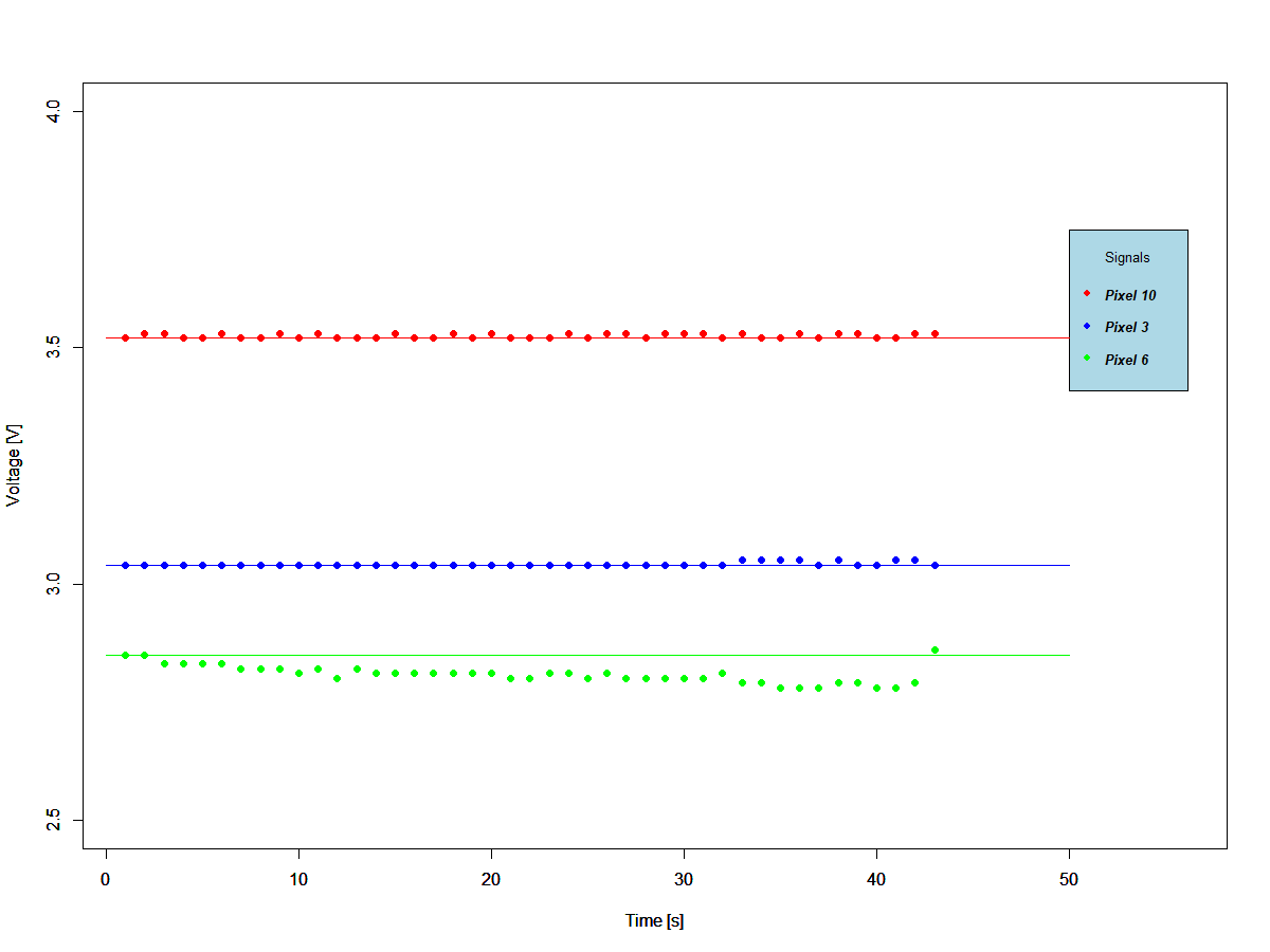
Time series

Finally, it was time to check whether the sensors could be drifting with time. The plot below shows consecutive reads of a fixed intensity value during around one minute.

The sensor measuring pixel 6 shows a large tendency to drift. Since this sensor controls the first decision tree split, the whole system is compromised at the outset. Nevertheless, this could not be the main issue since pixel 6 controls the identification of digit 1, and this has the best accuracy of all digits being identified.

ADC crosstalk

Finally, I checked whether the signals were affecting each other on the ADC and bingo. There was a huge effect of the signals on one another.

After a long day of unsuccessful troubleshooting the ADC cross-talk on the Arduino UNO, it was decided to simply reduce the microcontroller prototype to the identification of a single digit, i.e. no signal to cross-talk to. This would allow me to use my time more productively on the second prototype using discrete components which was the goal of this project.

Single digit decision tree using Arduino UNO

The final setup consisted of a single split and a single sensor,.

It looked straightforward enough but two out of the tree LDRs could not complete the tests. This because the drift and jitter were so large that after a few images, they'd go off the scale and stop measuring completely.

          [,1] [,2] [,3] [,4] [,5] [,6] [,7] [,8] [,9] [,10]
 [1,]       17    9    4    1    1    0    1    0    0     0
 [Not 1,]   10   13   15   22   14   16   20   15   23     0

The theoretical accuracy for number one obtained in the Minimum Model task was 60 %, whereas the accuracy obtained in this test was a few decimal points above 40 %. The result obtained with the prototype was not as good as I was expecting but OK considering the poor repeatability of the LDRs. 

Conclusion

The sensor choice proved to be unwise. They seemed to have a mind of their own and acted erratically at best.

The micro controller, in the hands of the inexperienced, could not rise to the challenge.

The model seemed to hold its own nevertheless despite the limitations. 

The next challenge will be to turn this concept finally onto a discrete-component object recognition system.