-
Minimum hardware
04/02/2020 at 22:37 • 0 commentsMinimum hardware
The goal of this task is to try and test minimum hardware solutions that can match the requirements of the project.
Minimum hardware is at best the most difficult part to define. The reason for this is that the objective of this project was also to try and have a high speed response, normally not compatible with the "minimum hardware approach". It's also the most difficult part for me to define since it's just really not my area. Nevertheless, I'll have a crack at at it and learn something along the way. That's what projects are for after all! In the meantime, forgive my many errors as I got trough this quest and let me know if there are better ways to implement this task.
So, in order to implement the simplest decision tree that was modeled using the data from the MNIST database in this project, I'd need a minimum of 13 pixels. Minimum pixel sensors, at hand, light dependent resistors, or LDR for short. These are reasonably cheap, widely available and can act as intensity sensors, readily able to measure the intensity of each pixel and translate it onto a voltage with a voltage divider.
Once the signal is ready, that's when the project becomes interesting since I have two types of solutions at hand, a Digital and an Analog solution.
Going digital
In order for the decision tree to be managed digitally, the information from the sensors would have to be received by an analog input and transformed onto a signal by an ADC. Now, there's quite a few micro controllers with 8 channels and then looking through the Mouser website I came across the PIC24 and PIC32 families with a whooping maximum of 122 IO, from which at most 32 IO cold be used as analog. Looking at the minimum model developed in the previous task, 32 analog inputs or pixels will not bring enough scale to the model, i.e. model scalability is hindered, and by limiting the model size, so is accuracy.
I know that digital signals can be multiplexed and then quite a few more IO signals could be accommodated but then we'd be adding layers to the system with time consuming operations. Bear with me, if possible, the goal is to have as simple a system as possible, even if that means capping the model to the available IOs.
Since this is not really my area of expertise and probably there are solutions out there with more than 32 analog inputs.
It does look like the most likely solution to a complex decision tree, and keeping with discrete component logic, the sensors would have to be multiplexed turned onto a digital signal in order to accommodate the large number of splits needed in the minimum 300-node decision tree model.
I'll call this the benchmark limit, to be upgraded once a new solution comes my way.
Going analog
Now, most of the information in this project is common knowledge, but for me most of it is eye-opening. For example, something as simple as turning a split in a decision tree onto a circuit was a mammoth task.
My first idea was to use transistors in a Schmitts trigger configuration. For those of you who know, it's obvious it'd never work since it has too much hysteresis and it just wouldn't switch if there were small differences in consecutive digits. So, first fail.
Second idea was to use transistors as Darlington pairs. My idea was to try and amplify the signal and create a split from "nested" pairs. This didn't work either since the voltage drop from consecutive pairs meant the after my second split, there was not enough voltage to do much at all. Second fail.
After shuffling trough some literature (ahem google), I came across the concept of voltage comparators. Yes, I know, for those of you who know... Well, for me it was an interesting trip down op-amp lane.
Well, the question is, can it beat an FPGA? That's a really hard thing to answer and I hope someone that knows what they're talking about can really help out here. Nevertheless, I'm going to go on a limb here and make some assumptions. For simplicity, the decision tree used for comparison will be one of the simple models from the minimum sensor log. Sensor speed will be assumed the same for both solutions.
![]()
Voltage comparator:
- The tree is 5 levels deep.
- The fastest comparators I could find had a minimum response time of 7 ns.
- Maximum response time, for the digits with 5 levels would be in the order of 35 ns.
High end FPGA:
- A fast ADC, like the MAX158BEAI+ has a sampling rate of 400kS/s with 8 channels, hence, we'd need two ADCs. Since the time is per channel, we could just brute-force it by using instead 11 single-channel ADCs. That caps the time to 2500 ns.
- The clock speed on a Stratix IV FPGA, claimed the world fastest, is 600 MHz, i.e. a cycle time, if everything runs on the same loop, of 1.6 ns. It doesn't really make a difference if we use one that is even faster, it's going to have to wait for the ADCs.
Conclusion
So, final solution, voltage comparators, LDRs, some resistors and LEDs of course to show which digit was detected. Can it get any simpler than that?
And the million dollar question, can a circuit built with voltage comparators beat an FPGA? In this case, and if my analysis is not too flawed, I'd say it beats the crap out of it. And it's a little bit cheaper as well.
Final step, prototyping.
-
Introduction
03/29/2020 at 12:45 • 0 commentsIntroduction
The typical machine vision systems I'm familiar with need to get the camera sensor data coded onto a protocol, transferred from the camera to the microchip, then decoded, and finally fed onto a pre-trained model which is solved by an IC, from which we can get a result.
The Nature paper describes an array of sensors which can be trained to recognize simple letters, i.e. it does the interpretation in the sensor array, forgoing most of the steps described above. The sensor array described in the paper is a complex setup well suited for a Research Institute but not so easy for a hacker to reproduce. At least for me to reproduce.
This was for me ML on the very edge, literally. I though that maybe something similar could be obtained with a simpler setup, using off the shelf parts, but also forgoing some of the steps typically needed for a machine-vision system.
My take on this was to try and make a prototype machine vision system that could identify images using discrete components by training a system based on decision trees. The sensors would be an array of photoresistors and the decision trees would be built using voltage comparators.
The training would all be carried out on a PC and the resulting decision tree implemented on an array of voltage comparators. The activation of the voltage comparator would be trimmed by adding resistors with the optical sensors to make voltage dividers which in turn would trigger the selection process.
There is a good possibility that this has been done in the past. If it has, I could not find anything similar.
Very quickly I realized two important things by looking at the dataset:
1. There would be some photoresistors' signal that would be ignored most of the time, i.e. my array would not be much of an array after all. It'd miss a few photoresistors. 2. Even if some photoresistors were missing, a simple array to analyse, e.g the MNIST number dataset would need an array of a few hundred photoresistors. I'm a father of 3 small kids with a full time job. This project quickly became impossible.
Then something came to my mind, what if I could simplify the pictures by averaging pixels? Would a lower definition picture reduce the efficacy of the decision tree?
The first objective was to develop some code to test this. All code was carried out in R using the RStudio IDE. Not extremely efficient but nice IDE I'm familiar with from previous forays on ML.
The target accuracy, in order to be at the level of a commercial solution, should be above 75%.
First decision tree
The first decision tree was produced using the rpart package and the full definition 28x28 digits and trained with the first 10000 images of the MNIST dataset. Below is a sample of a plot showing a digit represented by a single record on the MNIST matrix with all 28 x 28 = 784 "pixels". ```{r} image(avpic(2,1)) ```
After training the decision tree, the results were as follows:
## Decision tree: ```{r} rpart.plot(fitt, extra = 103, roundint=FALSE, box.palette="RdYlGn")
```
The confusion table below shows that a lot of numbers get miss-classified, but you only get what you pay for. If a better solution is desired, a neural network or a random forest will serve you well but at the expense of this project never seeing the light of day.
Confusion matrix
The diagonal shows how often the numbers are correctly identified. All the results outside the diagonal are miss-classified digits. Not looking so good. ```{r} table_mat ```
    0   1   2   3   4   5   6   7   8   9
0 349   5   2  10   8   7   0   4  31   0
1   1 346   8   7  34  19   0   8   6   7
2  48  22 215   4  12   6  15   6  42  25
3  23   6  33 239   6  35   2   7  47  21
4   1  10  13   7 277   8  11   6  12  40
5  47  10   5  28  32 155   5  10  54  14
6  36  24  31   0  63  12 186   4  32  11
7   1   3   4  16  34   4   0 326   9  22
8   6  23  27   7   9  13  13   1 241  43
9  10   9   3  46  28  12   2  52  18 205
Accuracy calculator
Ratio between the diagonal of the elements of the confusion matrix and the summation of the matrix and an indicator of how good the model is in classifying the digits.
```{r} accuracy_tune(fitt) ```
[1] 0.6352264
Accuracy for single digits
Similar to the previous metric but focused on single digits.
```{r} diag(table_mat)/apply(table_mat,1,sum) ```
        0         1         2         3         4         5         6         7         8         9
0.8389423 0.7935780 0.5443038 0.5704057 0.7194805 0.4305556 0.4661654 0.7780430 0.6292428 0.5324675
The accuracy of the system is not particularly good, and some digits fare much better than others.
Nevertheless, something became apparent. With 3 photo-resistors and 3 voltage comparators, the number 1 could be identified successfully eight out of ten times. And the whole system could be built with only thirteen photoresistors.
Comparison with a Random Forest
A comparison with a Random Forest trained model yields the following result:
Accuracy calculator
```{r} accuracy_tune(fittrf) ```
[1] 0.8100517
Accuracy for single digits
Similar to the previous one but focused on single digits. ```{r} diag(table_matrf)/apply(table_matrf,1,sum) ```
     0         1         2         3         4         5         6         7         8         9
0.8395270 0.9442351 0.7993448 0.7636512 0.7849829 0.7664504 0.9093904 0.8381030 0.7349823 0.7013946
With this model all digits fare much better than with the decision tree, but this solution cannot possibly be implemented in the way set out in this project. No easy way to implement 500 trees using discrete components.
Conclusion
The first calculations look promising. Further work is needed in order to verify the feasibility of this approach and confirm whether an extremely lean and extremely fast MNIST number recognition system can be built out of discrete components.
Acknowledgement
Below is a list of the giant's shoulders I remembered to reference. Sorry if there are more which this work relied upon and did not get referenced. Please inform me if you see part of your code above un-referenced and I'll correct the list below.
* Loading the MNIST dataset onto R and training with an SVM, https://gist.github.com/primaryobjects/b0c8333834debbc15be4
* RStudio Team (2015). RStudio: Integrated Development for R. RStudio, Inc., Boston, MA URL http://www.rstudio.com/.
* Nature's paper, https://www.nature.com/articles/s41586-020-2038-x
* Progress bar, https://ryouready.wordpress.com/2009/03/16/r-monitor-function-progress-with-a-progress-bar/
* Plotting and calculations on Decision trees, https://www.guru99.com/r-decision-trees.html
-
Minimum model
03/29/2020 at 09:41 • 0 commentsGoal
The goal of this task is to evaluate the best model for a discrete component object recognition system.
The first task would be to obtain a reference. Typical MNIST classifiers are well below 5% error rate (https://en.wikipedia.org/wiki/MNIST_database#Classifiers). We'll use a reference random forest, with no pre-processing on our reduced dataset.
Benchmark model
The dataset was reduced using the tools shown in https://hackaday.io/project/170591/log/175172-minimum-sensor and evaluated using the same metrics from the previous task.
Training the Random Forest does tax the system quite significantly. The training of a 10k dataset using parallel processing consumed all 8 cores of my laptop at full blast for a good few minutes.
The resulting random forest has the following characteristics:
- 500 trees
- Accuracy 83.6%
Considering that:
- The pixel density used was 4 x 4, instead of 28x28; and,
- Only 10k records were used and there was no pre-processing on the data, the fit is OK.
The fit for individual values was good and most digits were over 80%.
        0         1         2         3         4         5         6         7         8         9
0.8257426 0.8731284 0.9075908 0.8347743 0.8348018 0.8653367 0.9028459 0.8548549 0.7389061 0.7337058
Our aim is to make a model, based on decision trees, that could be implemented using discrete components that should match the accuracy of the random forest model.
Decision tree models
The choice of decision trees is due to the simplicity of this model with regards to its later implementation using discrete components.
Each split on a decision tree would take into account a single pixel and evaluated using discrete components.
By tuning the complexity parameters, we can increase the complexity of the tree in order to try and fit a decision tree that will approach the accuracy of the random forest.
The table below shows the effect on accuracy of the cp parameter:
      cp      Accuracy
 0.0010000000 0.6921987
 0.0005000000 0.7162860
 0.0003333333 0.7295383
 0.0002500000 0.7375396
 0.0002000000 0.7389565
 0.0001666667 0.7412902
 0.0001428571 0.7423737
 0.0001250000 0.7422904
 0.0001111111 0.7422904
 0.0001000000 0.7411235
The default cp parameter for the rpart package in R is 0.01 and with successive iterative reduction we obtain no visible increase in accuracy with cp below 0.00025 and we're still quite a way away from the target accuracy obtained with the random forest.
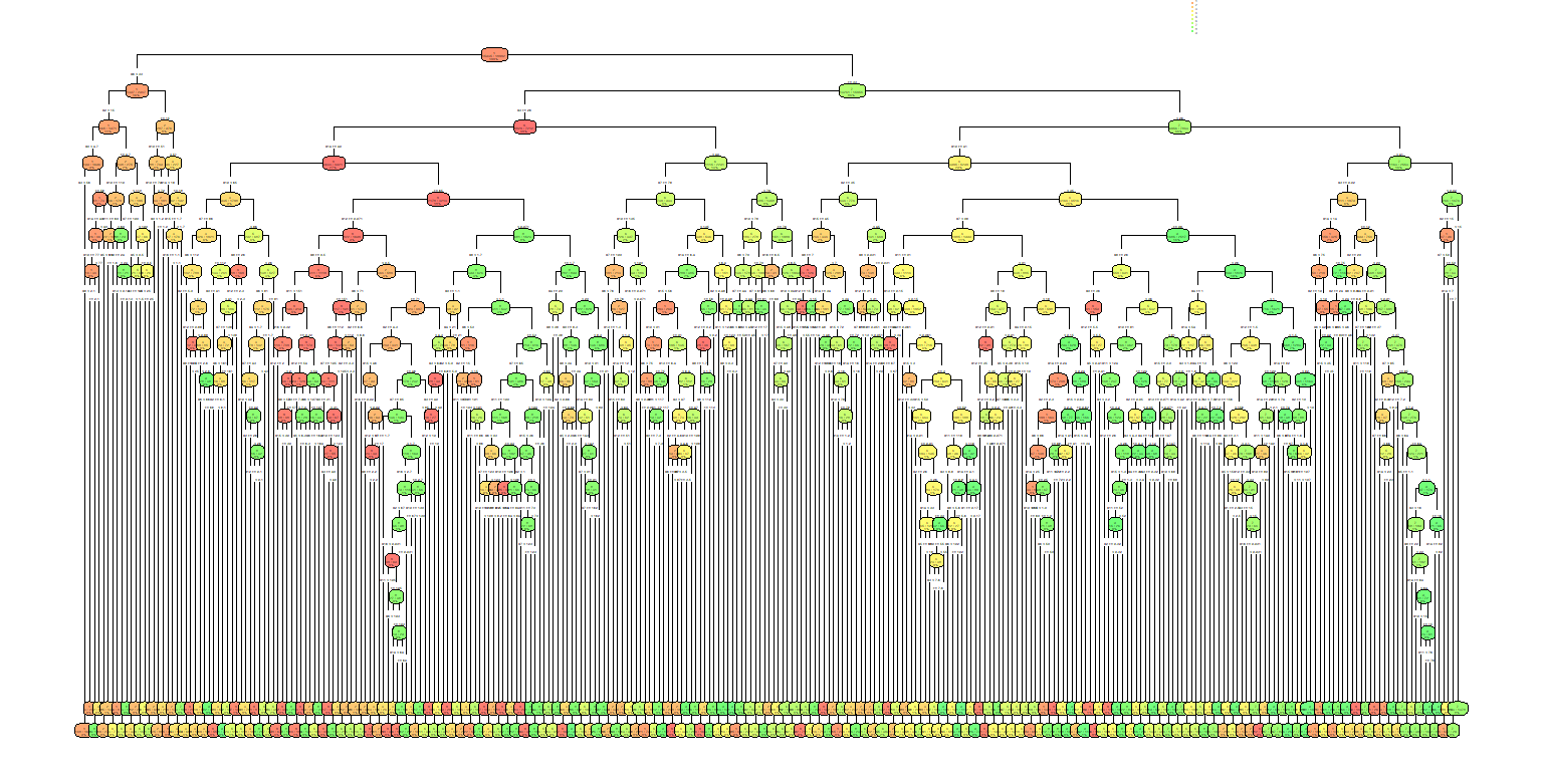
Even settling for a cp of 0.0025, assuming there's a limit on what can be achieved with decision trees, the result is mindboggling. The resulting tree has a total of 300 nodes or splits.
Could it be implemented using discrete components? Definitely. Maybe.
![]()
Conclusion
Decision trees can achieve a reasonable accuracy at recognizing the MNIST dataset, at a complexity cost.
The resulting tree can reach a 73% accuracy which is just shy of the 75% target we set out in this project.
-
Minimum sensor
03/27/2020 at 23:53 • 0 commentsGoal
The goal of this task was to evaluate how simple a sensor array would be needed to reach object recognition on the MNIST database to a commercial level accuracy.
According to this site, commercial OCR systems have an accuracy of 75% or higher on manuscripts. Maybe on numbers they do better but we'll keep this number as our benchmark.
So there are two ways to test the minimum pixel density needed o identify the MNIST database with 75% accuracy:
1. Grab a handful of sensors, test them against the same algorithm and benchmark them. Time consuming and beyond my budget and time allowance.
2. Try and train a simple object recognition algorithm with a database that reduces in pixel density. Now, that's up my beach.
The algorithm of choice was an easy sell. Since I'm focusing on the lowest denominator, decision trees it is.
Experimental
The database was obviously the MNIST database, the model was a standard decision tree with the standard parameters included with the rpart package in R.
The database was loaded using the code from Kory Beckers GIT project page https://gist.github.com/primaryobjects/b0c8333834debbc15be4 and the matrix containing the data was transformed by averaging neighboring cells as below. Code snippets can be found in the last section. Full code to be uploaded as files.
This is the original 28 x 28 matrix image showing a zero.
![]()
By applying a factor of 2, the matrix becomes a 14x14. Still quite OK.![]()
By applying a factor of 4, the matrix became a 7x7 matrix. We humans could have still told this used to be a zero, if you made an effort.
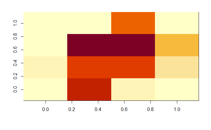
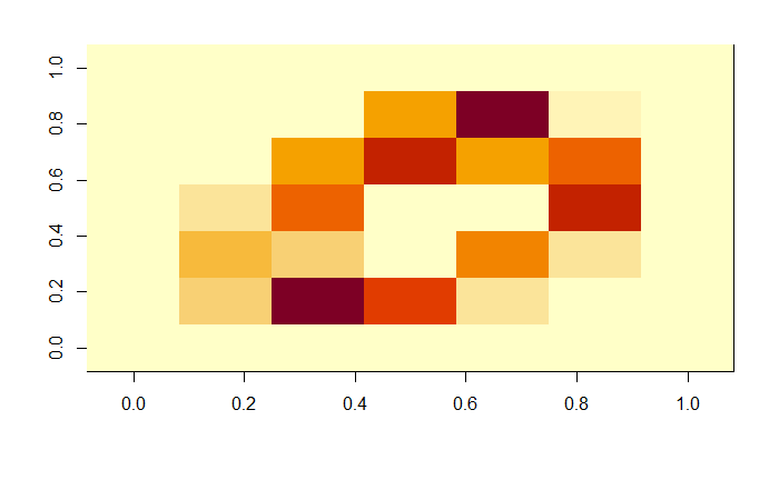
![]() Now what happens when the matrix is reduced by a factor of 7? Is the zero still recognizable? It's really a hard call. It may as well be a one at an angle, or a four. I chose to keep an open mind since I didn't really know how far the algorithm could see things that I couldn't.
Now what happens when the matrix is reduced by a factor of 7? Is the zero still recognizable? It's really a hard call. It may as well be a one at an angle, or a four. I chose to keep an open mind since I didn't really know how far the algorithm could see things that I couldn't.![]()
Finally, the last factor was 14, i.e. the initial 28x28 matrix was averaged to a 2x2. This would be a really poor sensor, but I needed to find the point at which the model couldn't tell the numbers apart and then start going up in pixel density.
![]()
Modelling
Once the matrix datasets were ready, it was time to see how the lower resolution pictures fared versus the full resolution database when pitched against the standard decision trees using a 10000 record training set.
So, the images could be simplified and the number of pixels reduced by averaging them. The decision tree model had already shown a piss poor accuracy for starters. Less pixels might not affect it much. So let's see how they fared.
As a reference, the full 28x28 matrix with the standard decision tree had the following results:
Overall model accuracy (defined as the sum of the confusion matrix diagonal divided by the total number of tests)
0.6352264

Individual digit accuracy (Obtained by dividing the number of times the number was correctly identified versus the number of times the model thought it recognized the number)
         0         1         2         3         4         5         6         7         8         9
0.8389423 0.7935780 0.5443038 0.5704057 0.7194805 0.4305556 0.4661654 0.7780430 0.6292428 0.5324675
That is to say, 63% of the times it got the number right. Some digits like 0, 1, 7 and 4 fared quite well, whereas the other ones didn't really make the cut. Let's keep an open mind nevertheless, a monkey pulling bananas hanging on strings would have gotten 10%. The model is doing something after all.
14 x 14 dataset
There was a clear improvement in classification for all digits with a marginal improvement for the overall accuracy, i.e. less pixels gave a better classification criteria.
This is the equivalent of going out to the pub and starting to see clearer after a few pints. I'm pretty sure our brains have decision trees and not neural networks.
Overall model accuracy

0.6667501
Individual digit accuracy
        0         1         2         3         4         5         6         7         8         9
0.8689320 0.8491379 0.5525606 0.5892421 0.5493671 0.4624277 0.5859564 0.8186158 0.5795148 0.7304786
7 x 7 dataset
Accuracy was very similar to the full 28x28 matrix.
At this point things got interesting. I was not expecting the decision tree to fare very good at this stage. All in all, the model was extremely simple an the results not really that much worse than the original matrix. This is with a 2^4 reduction in information density.
Overall model accuracy
0.635977

Individual digit accuracy
    0         1         2         3         4         5         6         7         8         9
0.6223278 0.8741573 0.4199475 0.6247031 0.6057441 0.4382353 0.6942529 0.6253102 0.6129032 0.7702020
4 x 4 dataset
The decision tree built with the default configuration was significantly simplified. We were still able to detect number 1 with three pixels and at an acceptable accuracy for something this simple.
The overall accuracy went down significantly at this point, which is not surprising. What was surprising was that the accuracy of the model was much better than whatever I was expecting it to achieve. If you've seen a picture of the variation in shape and angle of the MNIST database, you'd appreciate a decision tree that can tell the numbers apart 50% of the time with just 4 pixels by 4 pixels.
Overall model accuracy
0.5596698

Individual digit accuracy
        0         1         2         3         4         5         6         7         8         9
0.5758294 0.7523148 0.4809160 0.3478261 0.4987893 0.2529762 0.7615572 0.7587007 0.5405405 0.5351759
Numbers 1, 3 and 7 could be identified successfully over 75% of the times. Honestly, at this pixel density, it all looked the same to me.
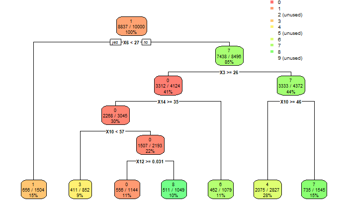
Now, in order to appreciate how simple this system is, attached below is the decision tree generated using the 4 x 4 matrix.
![]()
In order to properly classify the number 1, I'd need 3 pixels. For number 7, I'd need two extra pixels. For number 6, another three pixels on top of the two needed to identify number 7. That's a total of 8 pixels in order to identify 3 digits with a 75% accuracy. Now, that is really cool.
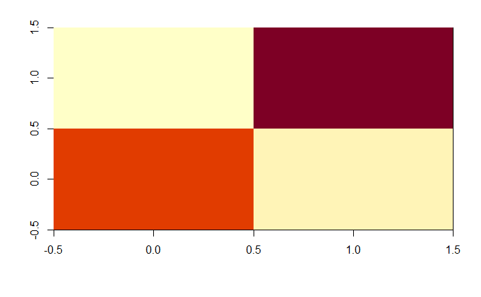
Just for reference, this is what a 4x4 zero looked like:
![]() I didn't even bother with the 2x2. I was already happy.
I didn't even bother with the 2x2. I was already happy.Prototyping
So now, before I turned this onto a product I could sell, I needed to prototype it. My go-to prototyping tool was an Arduino Uno. As pixel sensors I settled for LDRs. The reason for this was I had nothing else laying around.
In the Arduino there are only 6 analog inputs so the decision tree had to be simplified even further. For this, we could try and adjust the complexity parameter (cp, see https://www.rdocumentation.org/packages/rpart/versions/4.1-15/topics/rpart for details) in the decision tree in order to get a more palatable solution with 6 or less splits.
Since there was no single solution that could give me a good number of splits with an acceptable accuracy result for all the digits, I decided to compromise and settle for only some digits instead. This was a proof of concept after all.
With a low enough complexity parameter I could get a decision tree that would allow me to identify 3 numbers with an accuracy of over 70% with only 5 pixels, in my 4x4 simplified array.
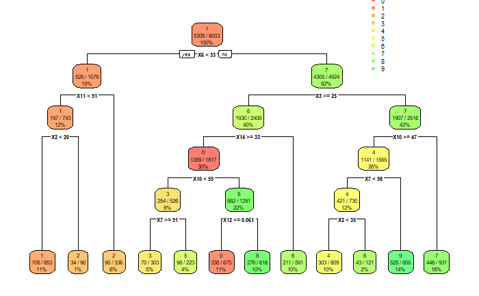
So now it came to building the prototype. So whilst I tried to gather my pixel sensors, I realized that I only had 3 LDRs. Well, time to compromise again. If I reduced the complexity parameter even further, the decision tree became incredibly dumb. I then tried to train the model with a larger dataset. This gave me the decision tree shown below. With 3 pixels I could identify three numbers with an acceptable accuracy.
![]()
The decision tree is nevertheless ignoring numbers 2, 5 and 9. Don't let "perfect" be the enemy of "some of it works".
The confusion matrix for the above model is attached below.
       0    1    2    3    4    5    6    7    8    9
  0  911    1    1    0  204    0   59   30    0    0
  1   35 1013   33    0   68    0   66  141    0    0
  2  275  136  413    0  196    0  136   14    0    0
  3  656   35  153    0  177    0   32  183    0    0
  4   16   39    0    0  929    0  118   61    0    0
  5  509   18    1    0  387    0   84  113    0    0
  6  124   24    5    0  268    0  757    2    0    0
  7   16   25   20    0  286    0    3  874    0    0
  8  696   36    1    0  241    0  143   22    0    0
  9   60    4    0    0  882    0   48  218    0    0
The overall accuracy of the model is just over 40%, well shy of the 75% target, but its objective is to validate the concept.
The best accuracy for the individual digits is for numbers 1, 4 and 7, with 60%, 24% and 43% respectively.
Conclusion
The goal of this task was successfully achieved.
- We have a minimum sensor requirement.
- We have a minimum model.
- We have a prototyping platform.
- I have a newly found respect for decision trees.
Next, the Minimum model.
Discrete component object recognition
Inspired by a recent paper, the goal is to develop a system that can recognize numbers from the MNIST database without a microcontroller

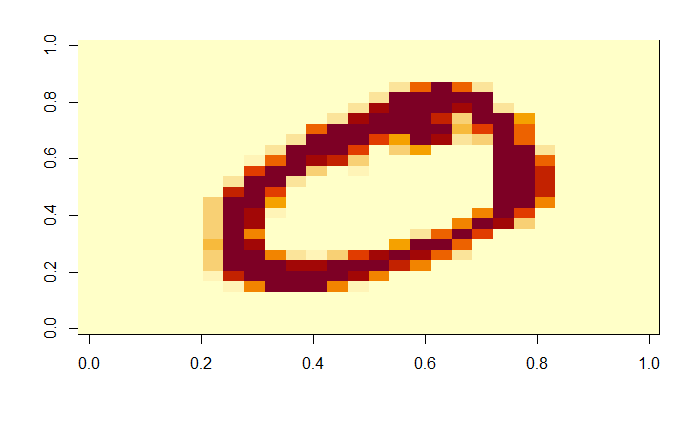
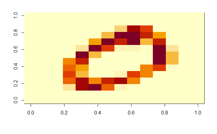
 Now what happens when the matrix is reduced by a factor of 7? Is the zero still recognizable? It's really a hard call. It may as well be a one at an angle, or a four. I chose to keep an open mind since I didn't really know how far the algorithm could see things that I couldn't.