Supplyframe DesignLab
-
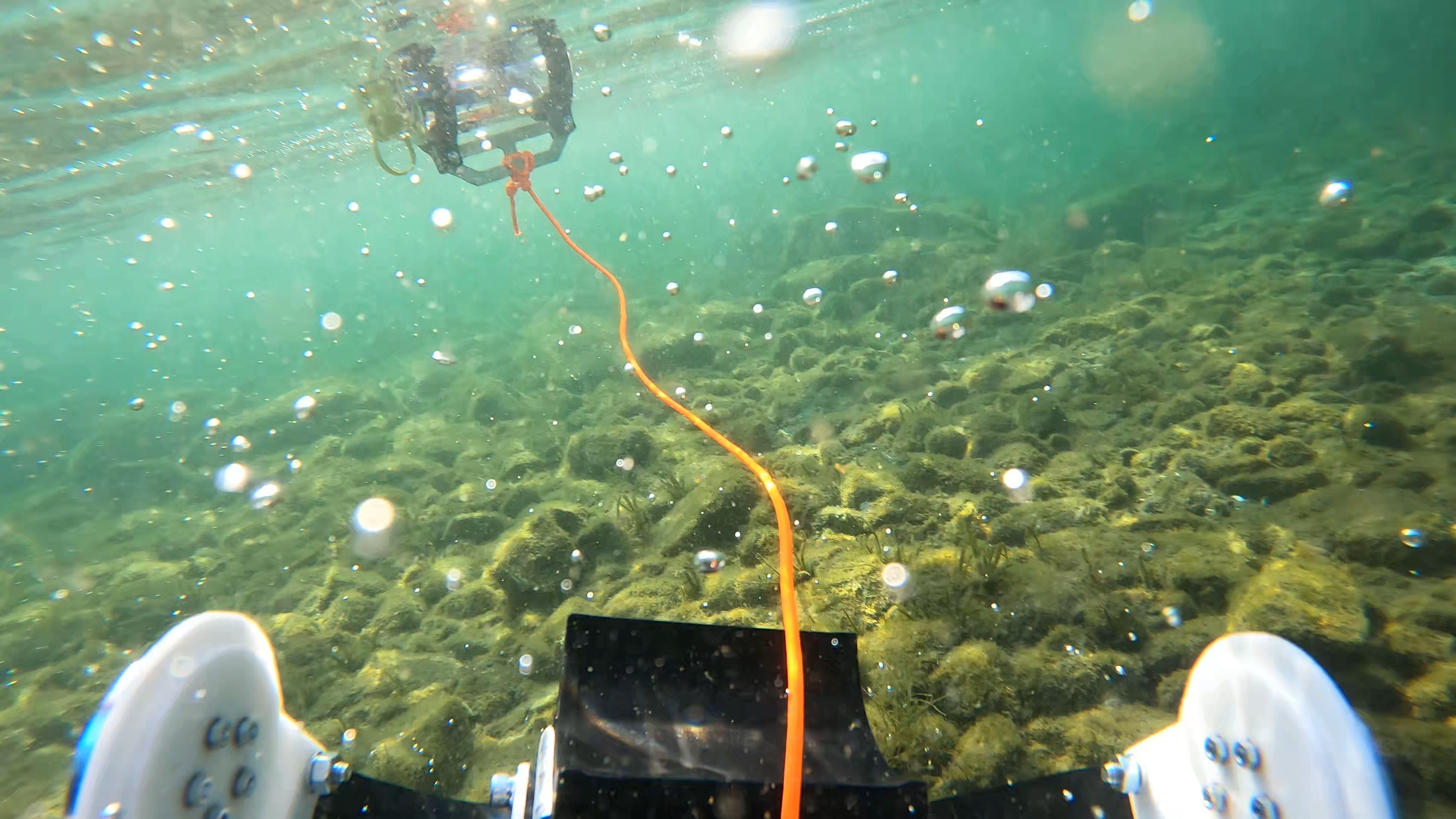
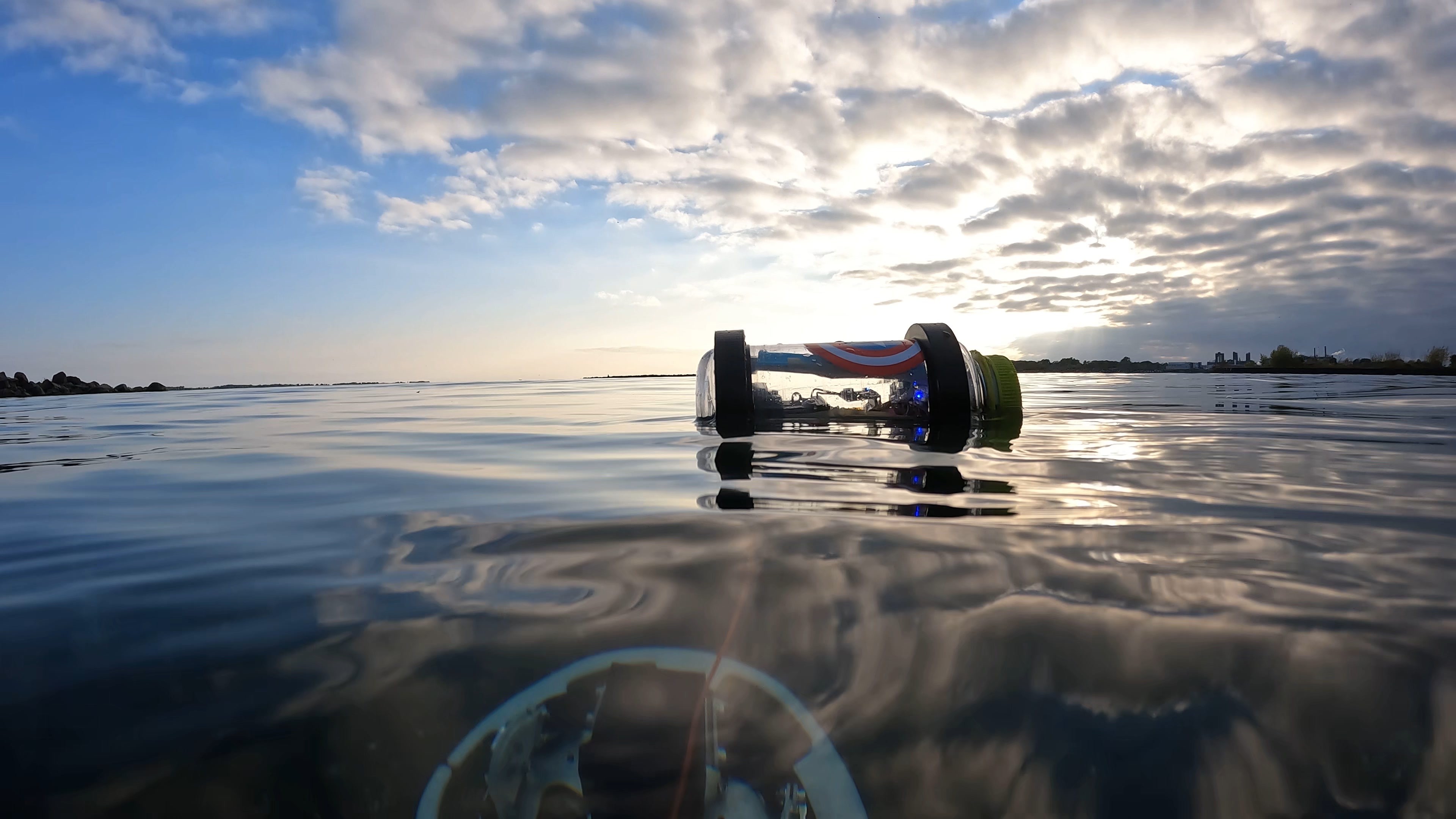
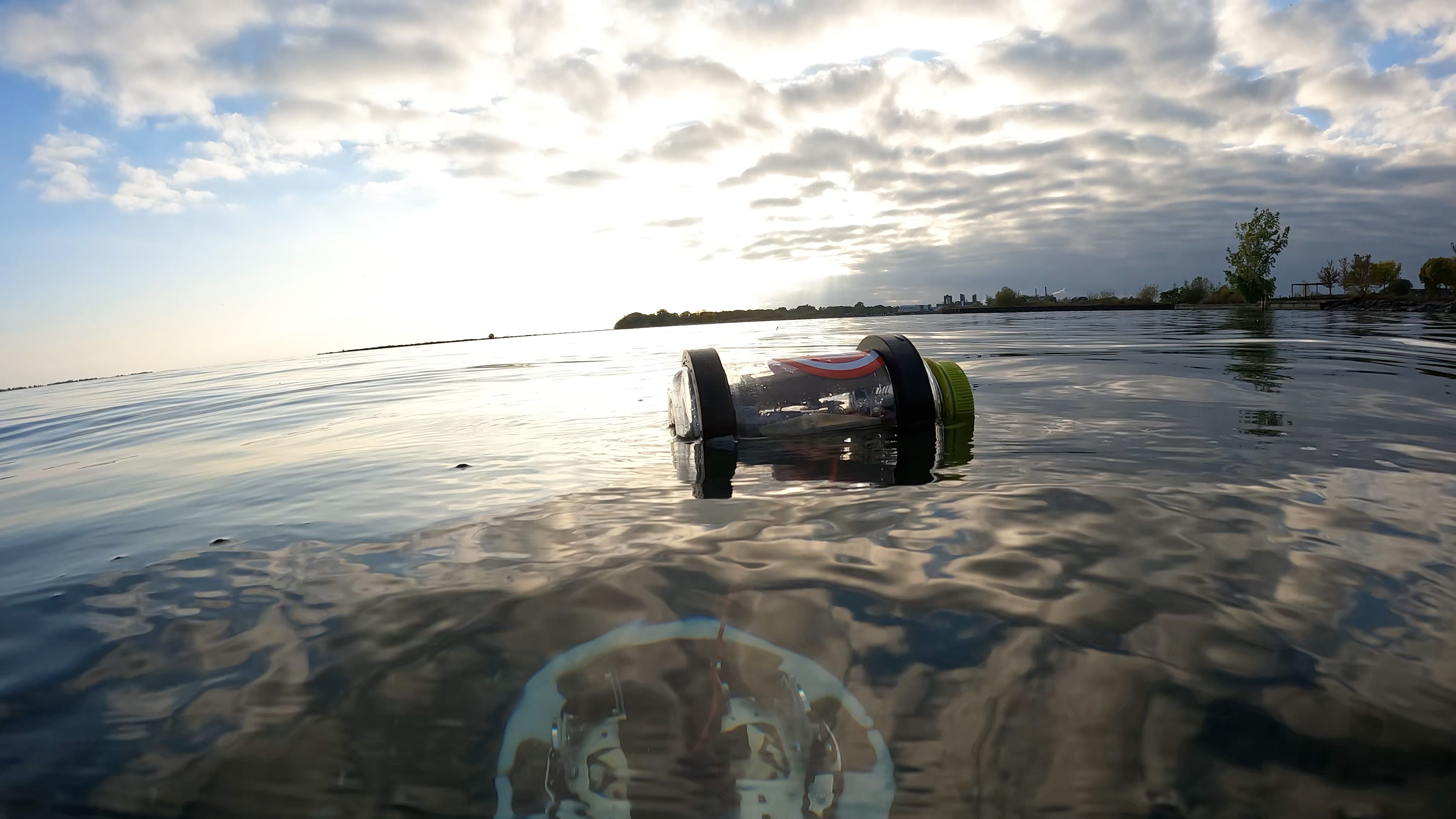
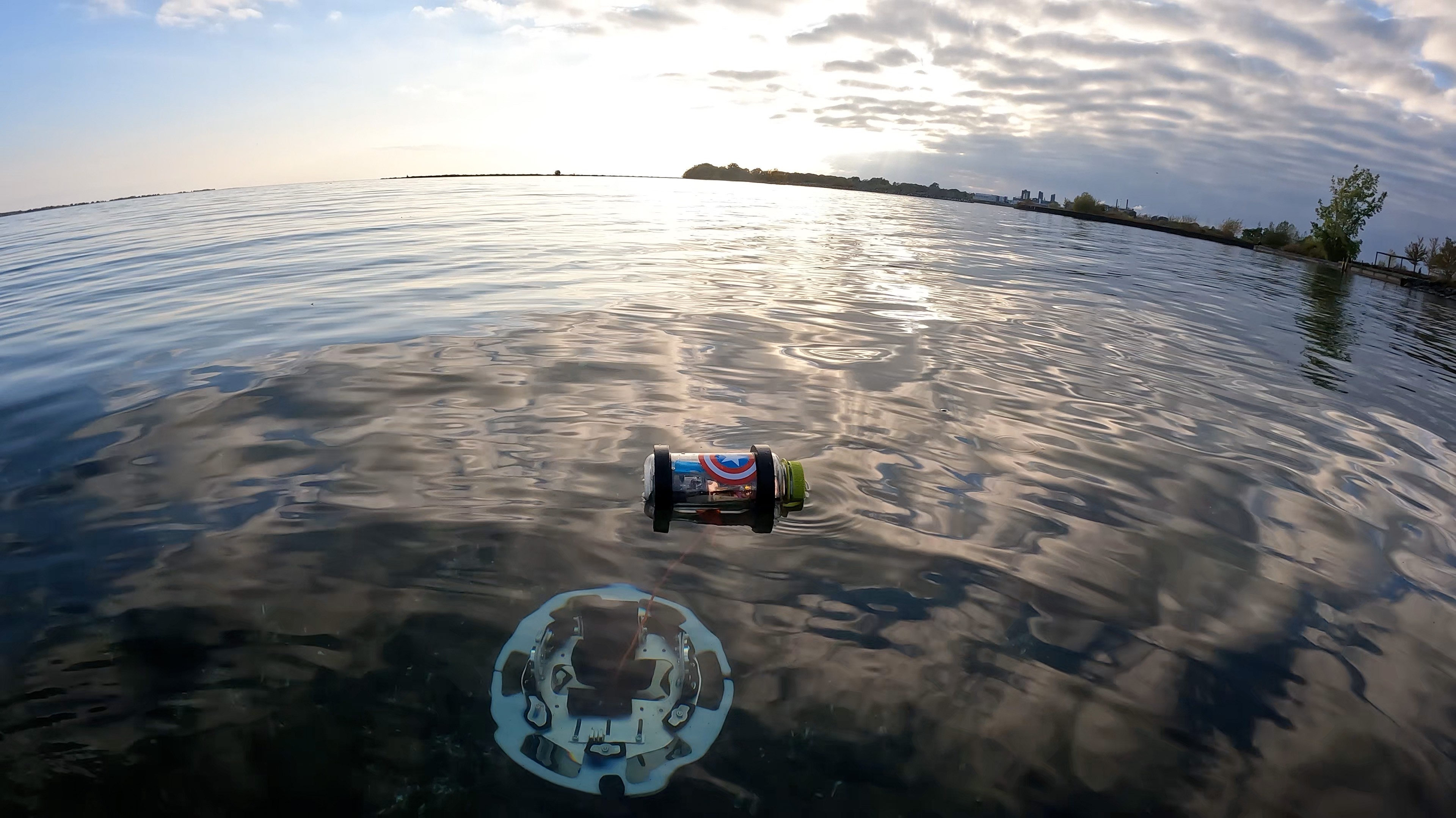
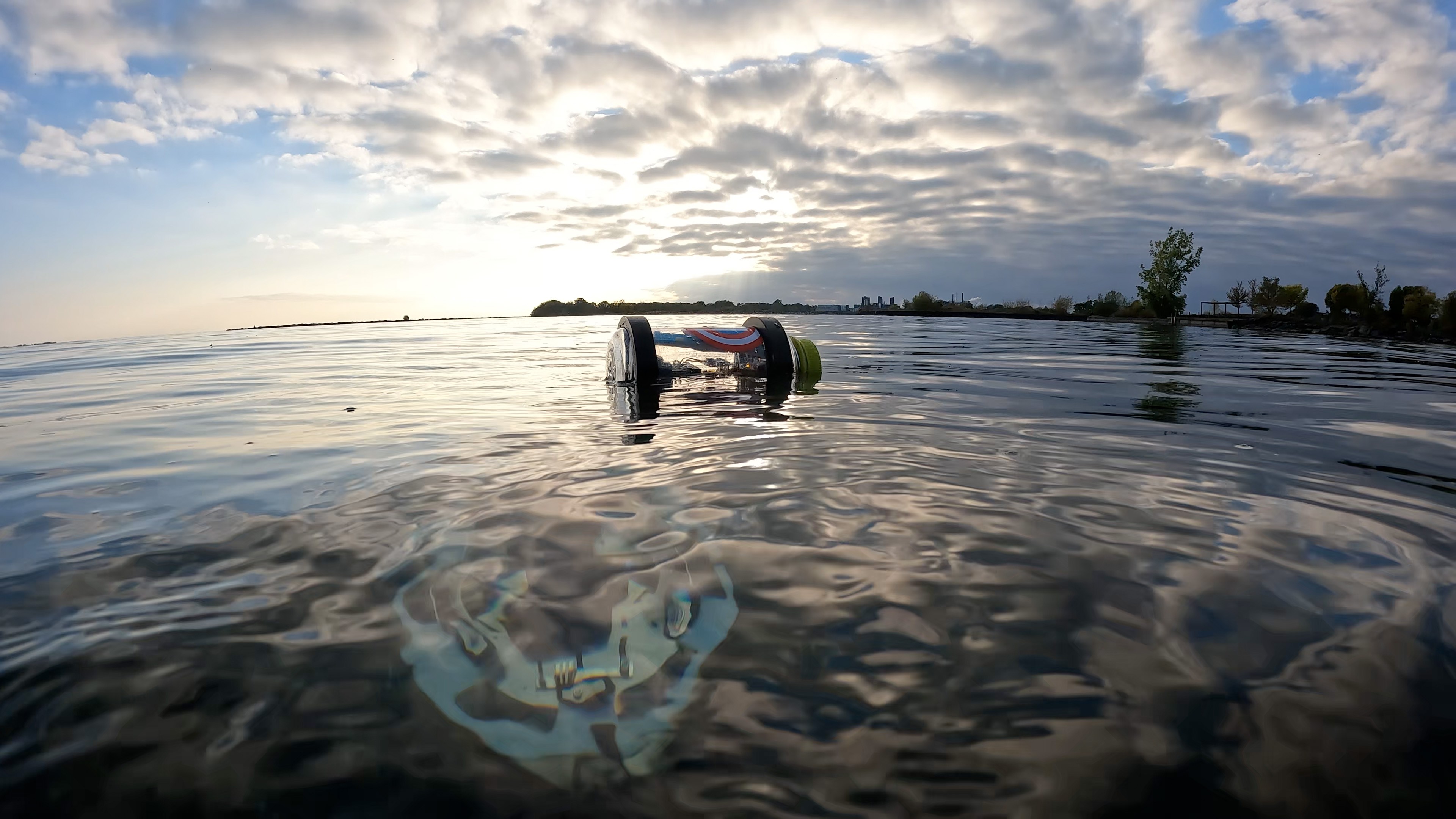
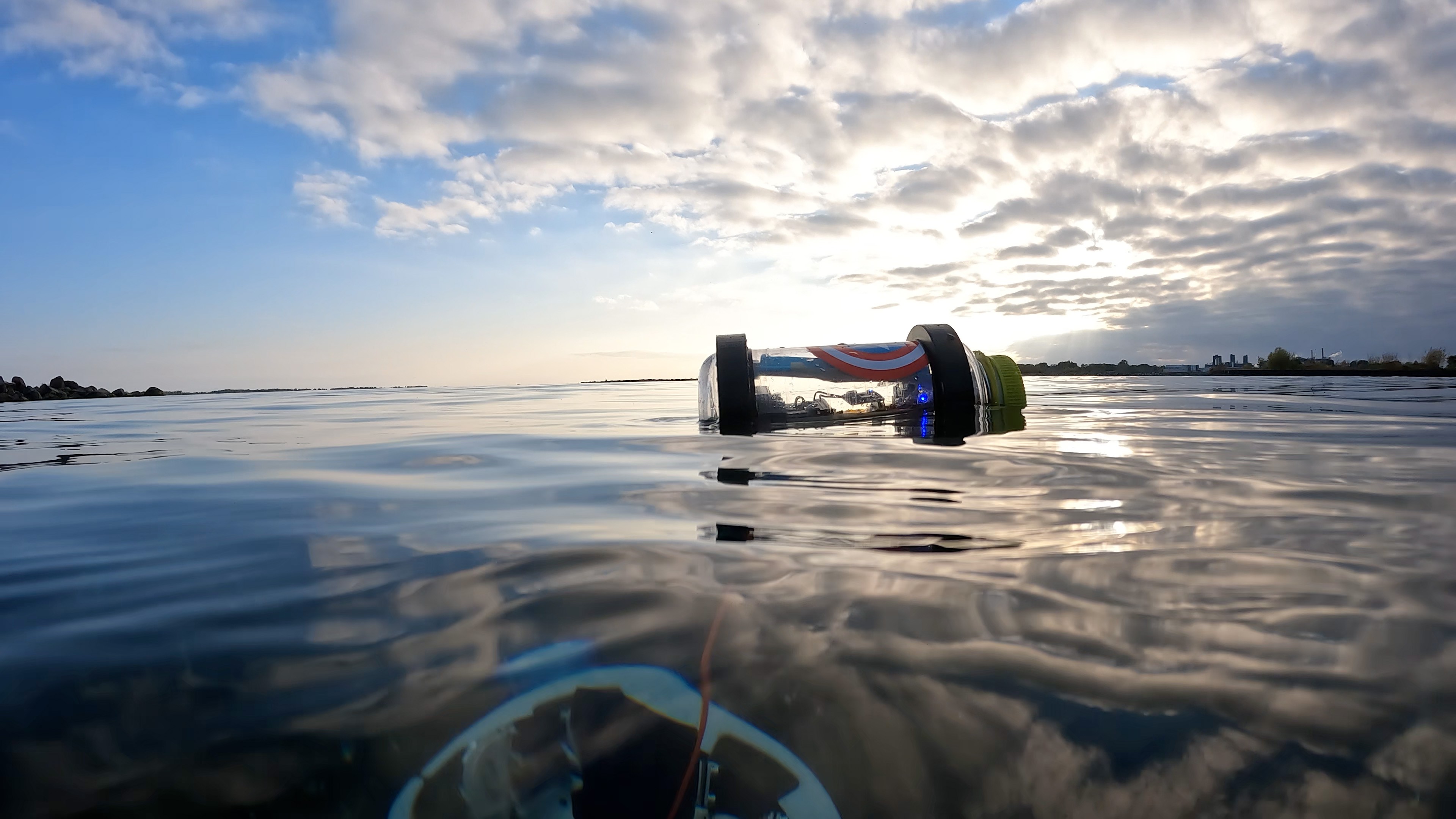
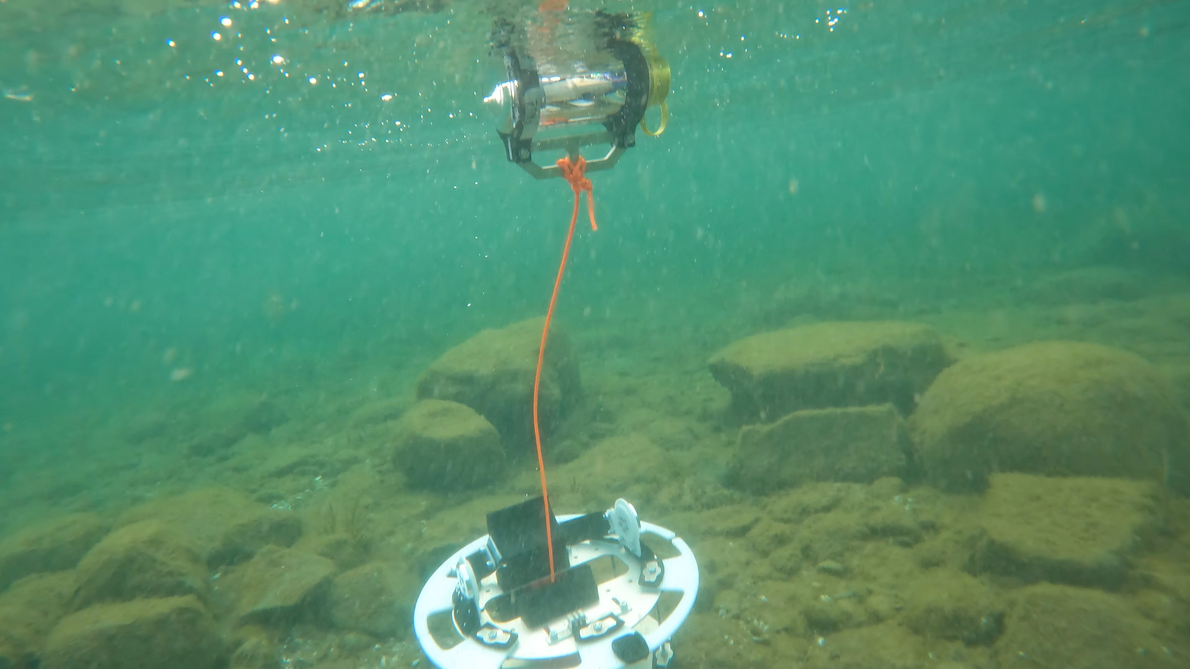
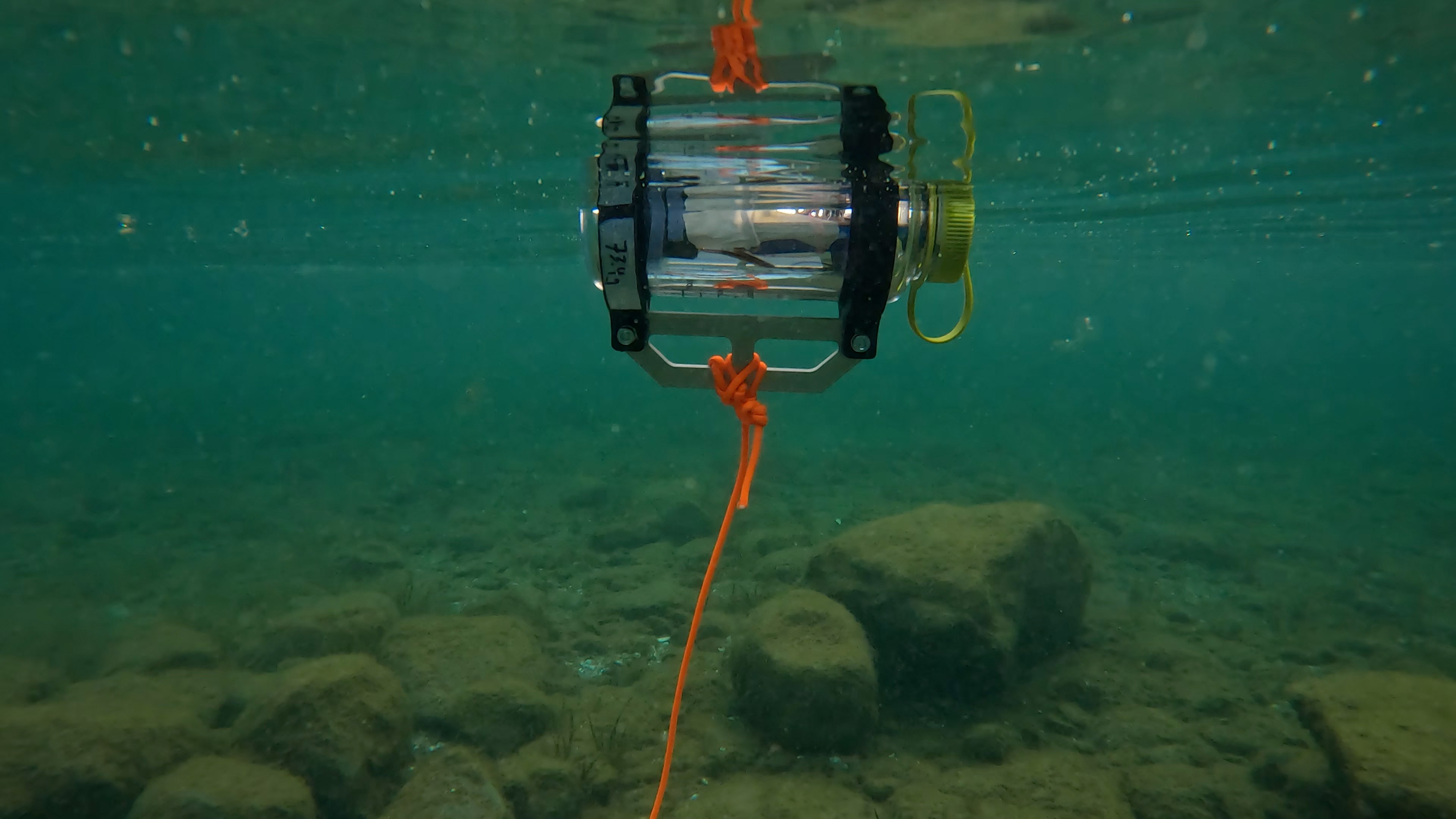
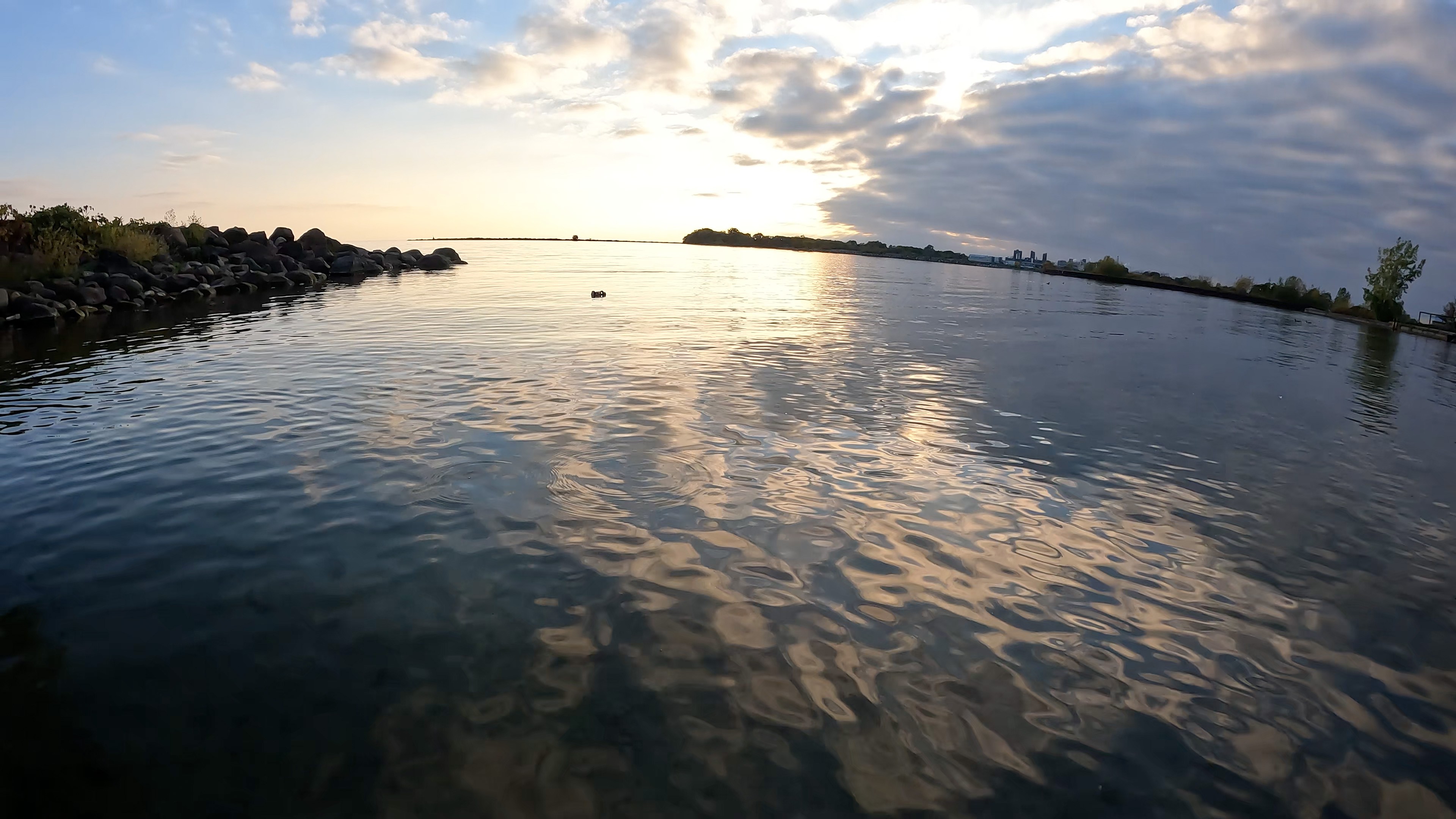
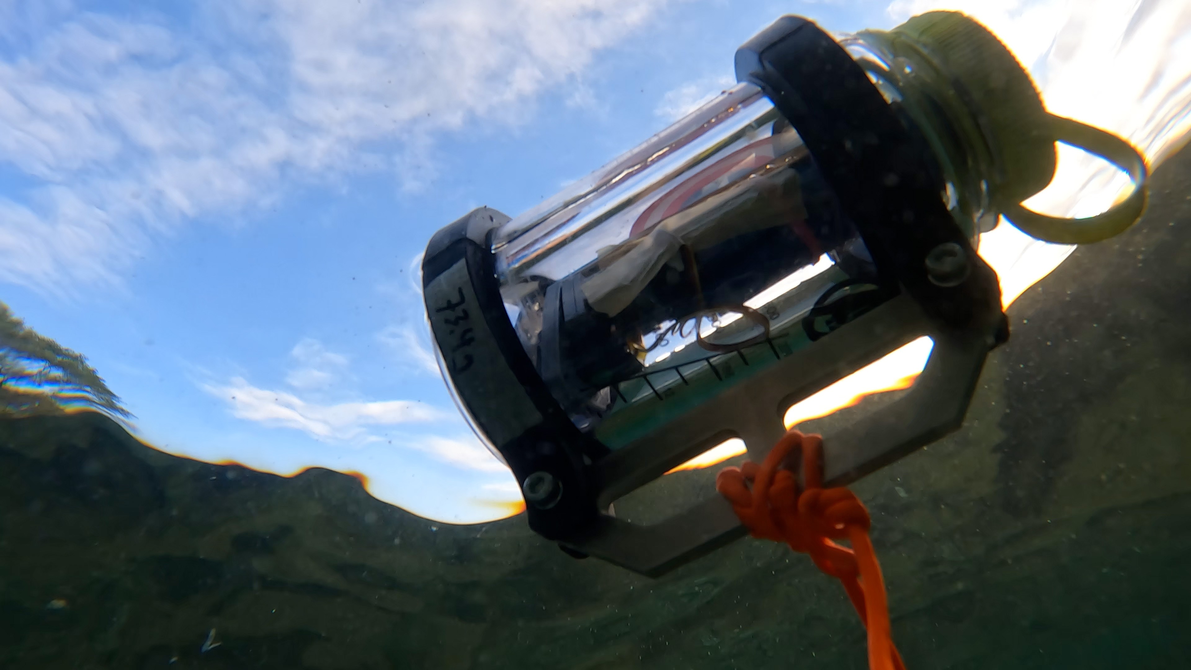
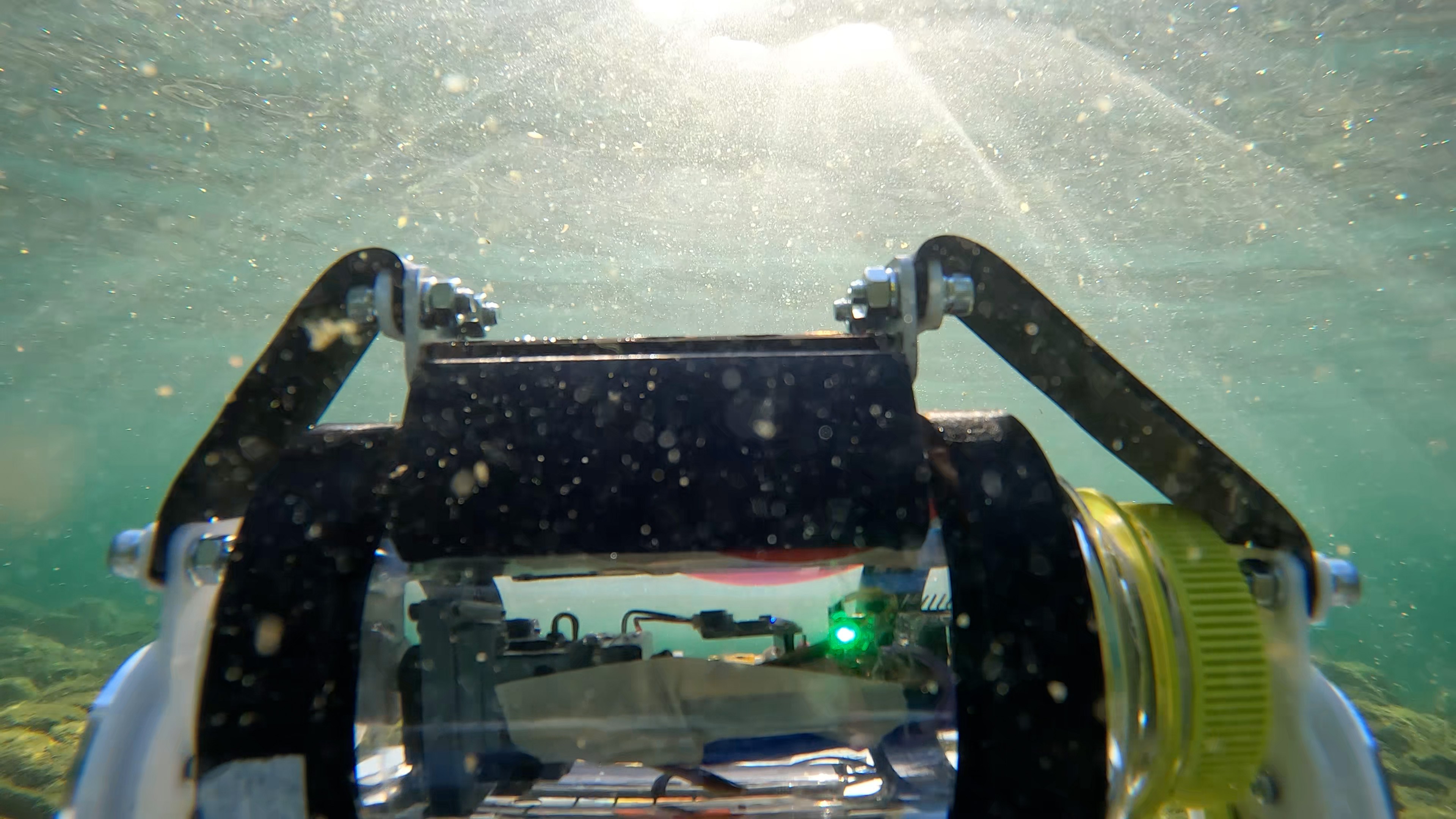
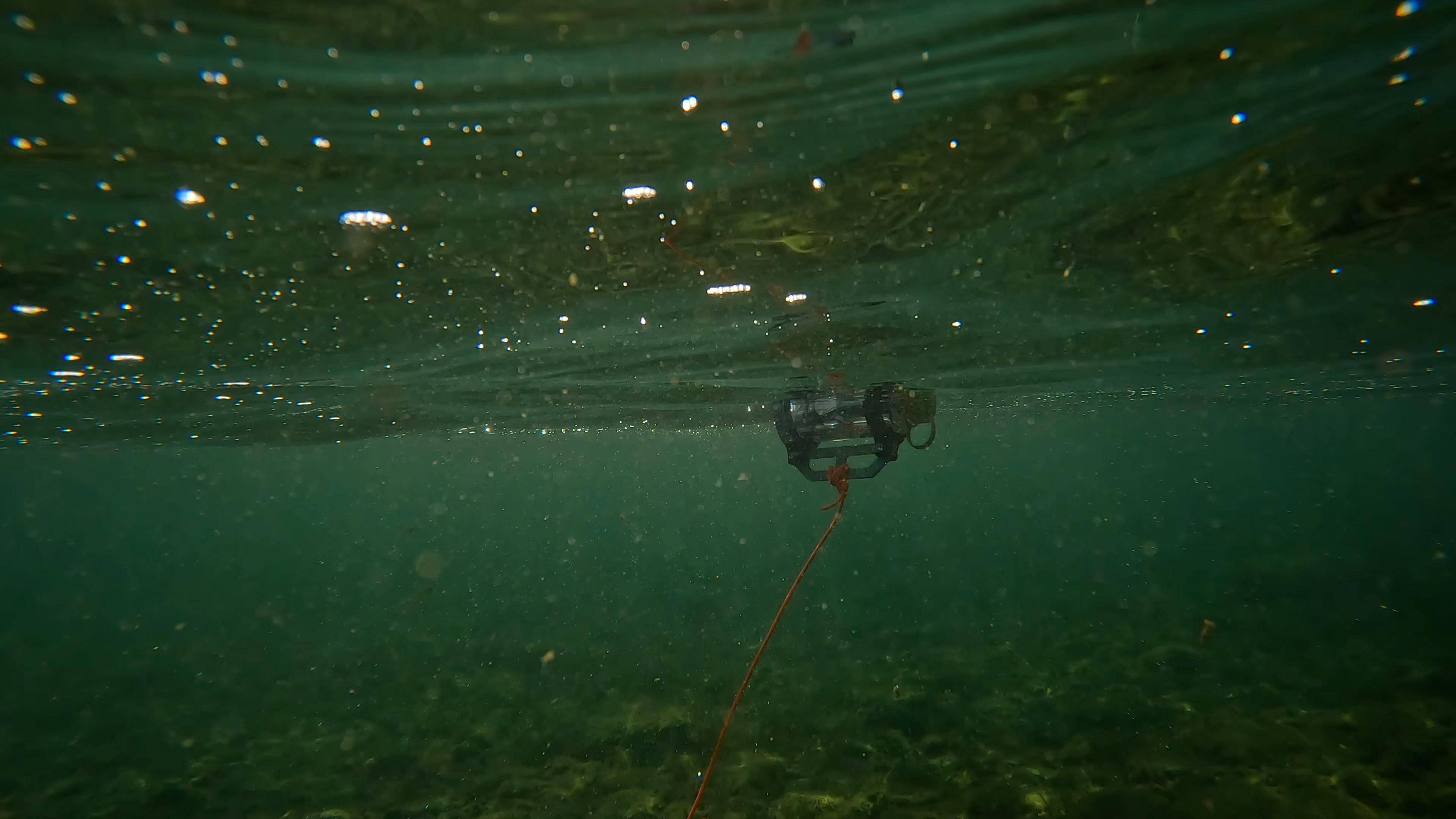
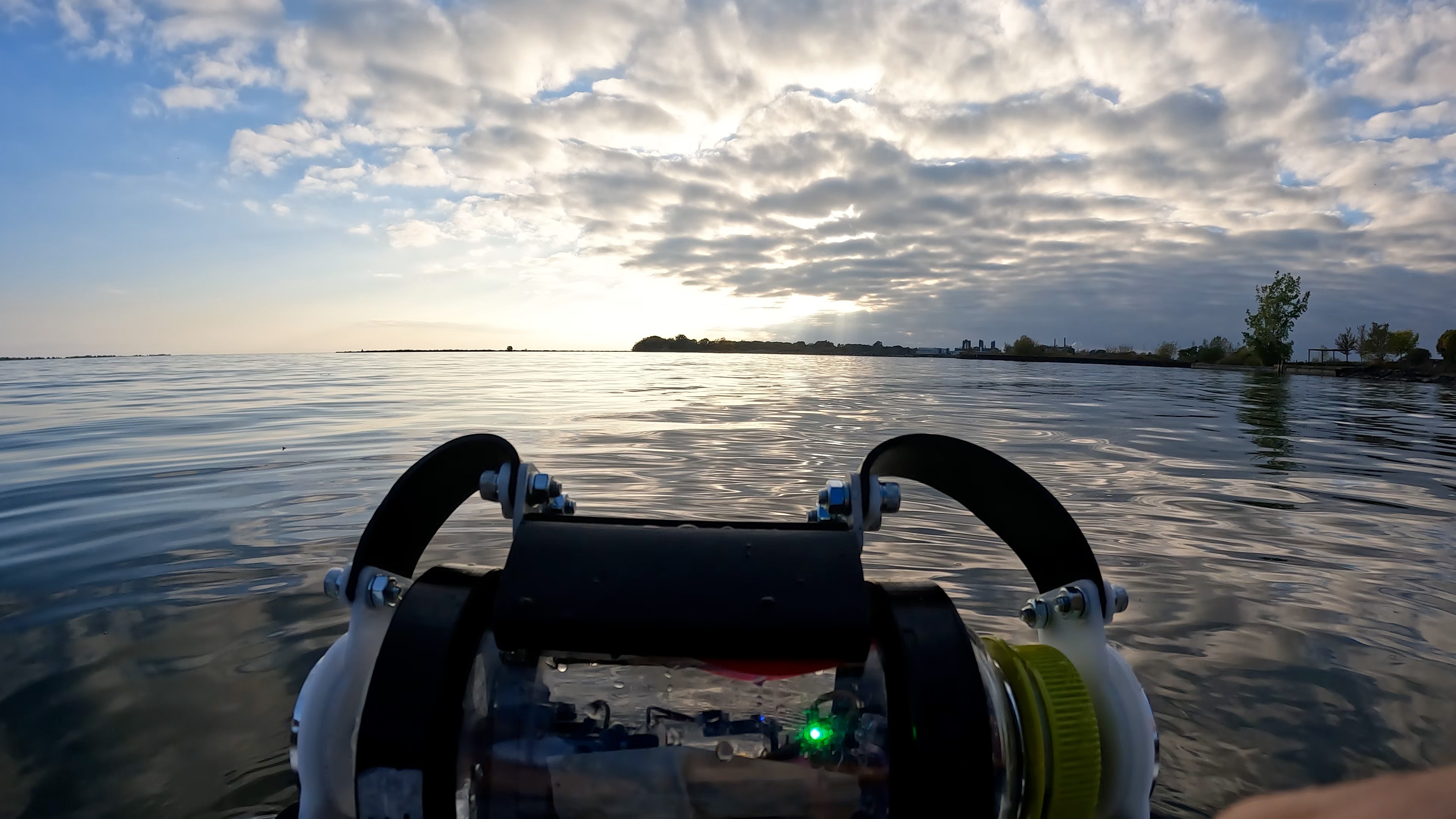
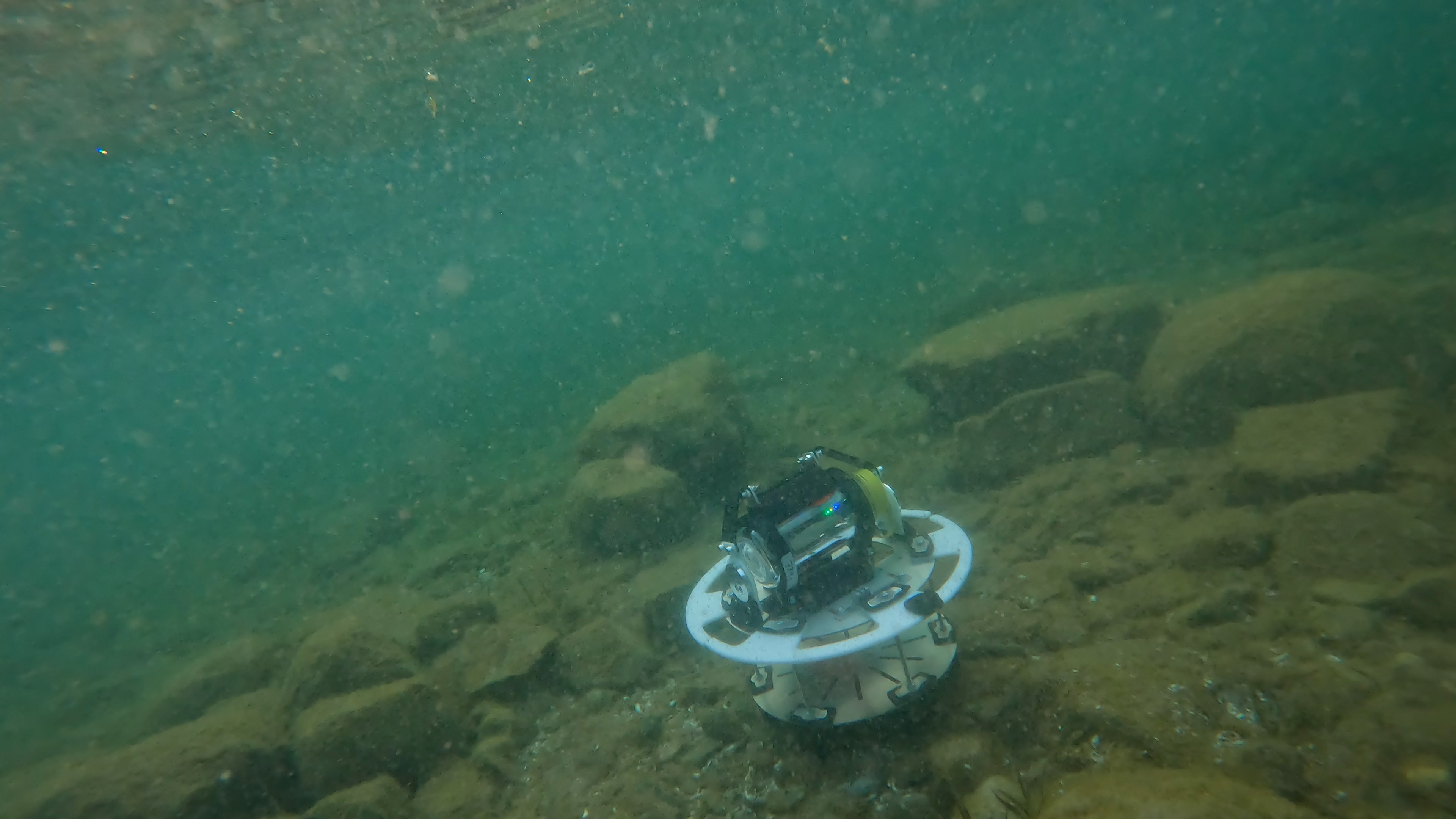
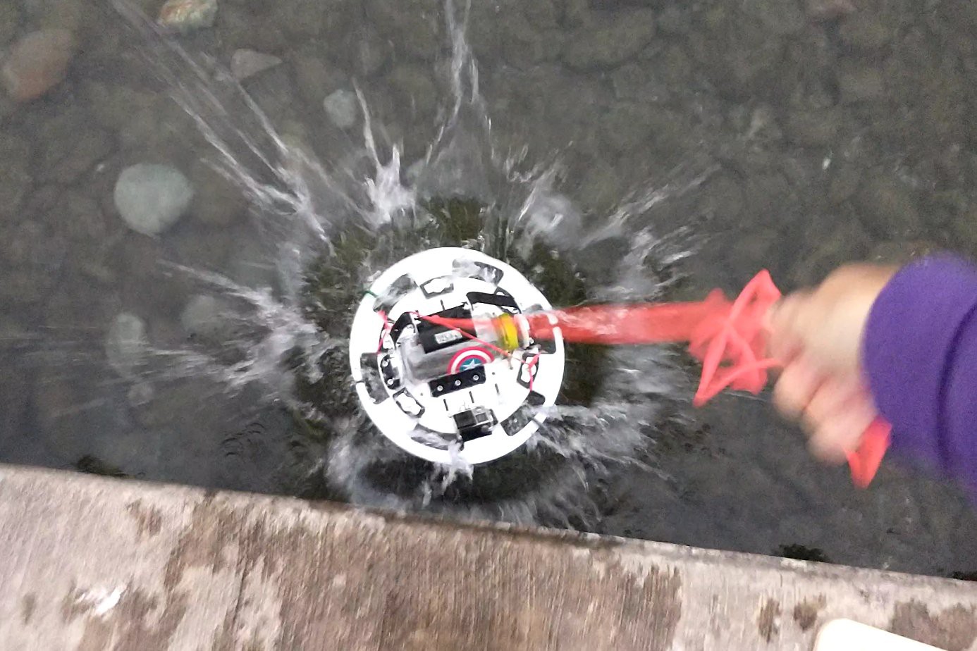
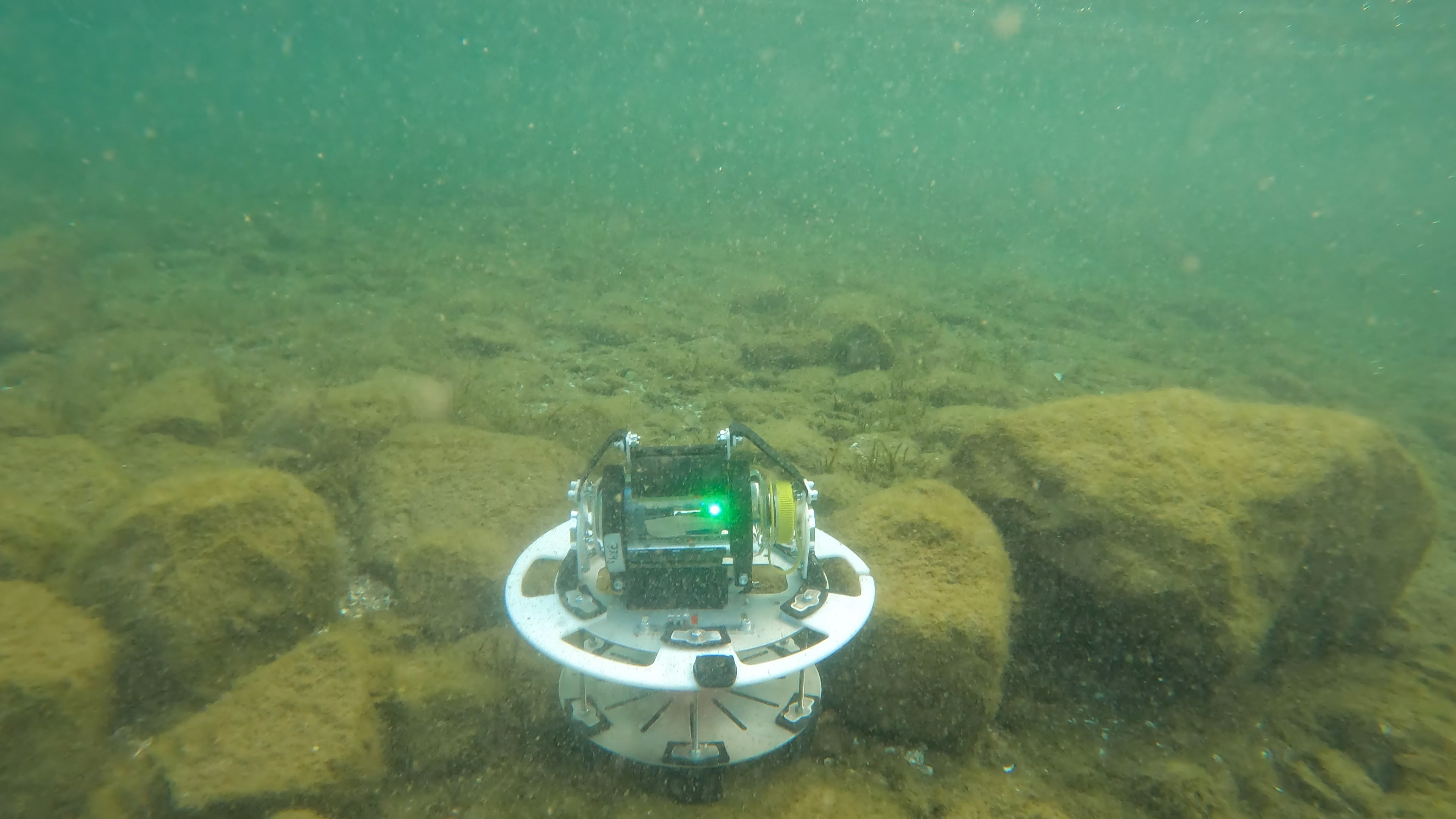
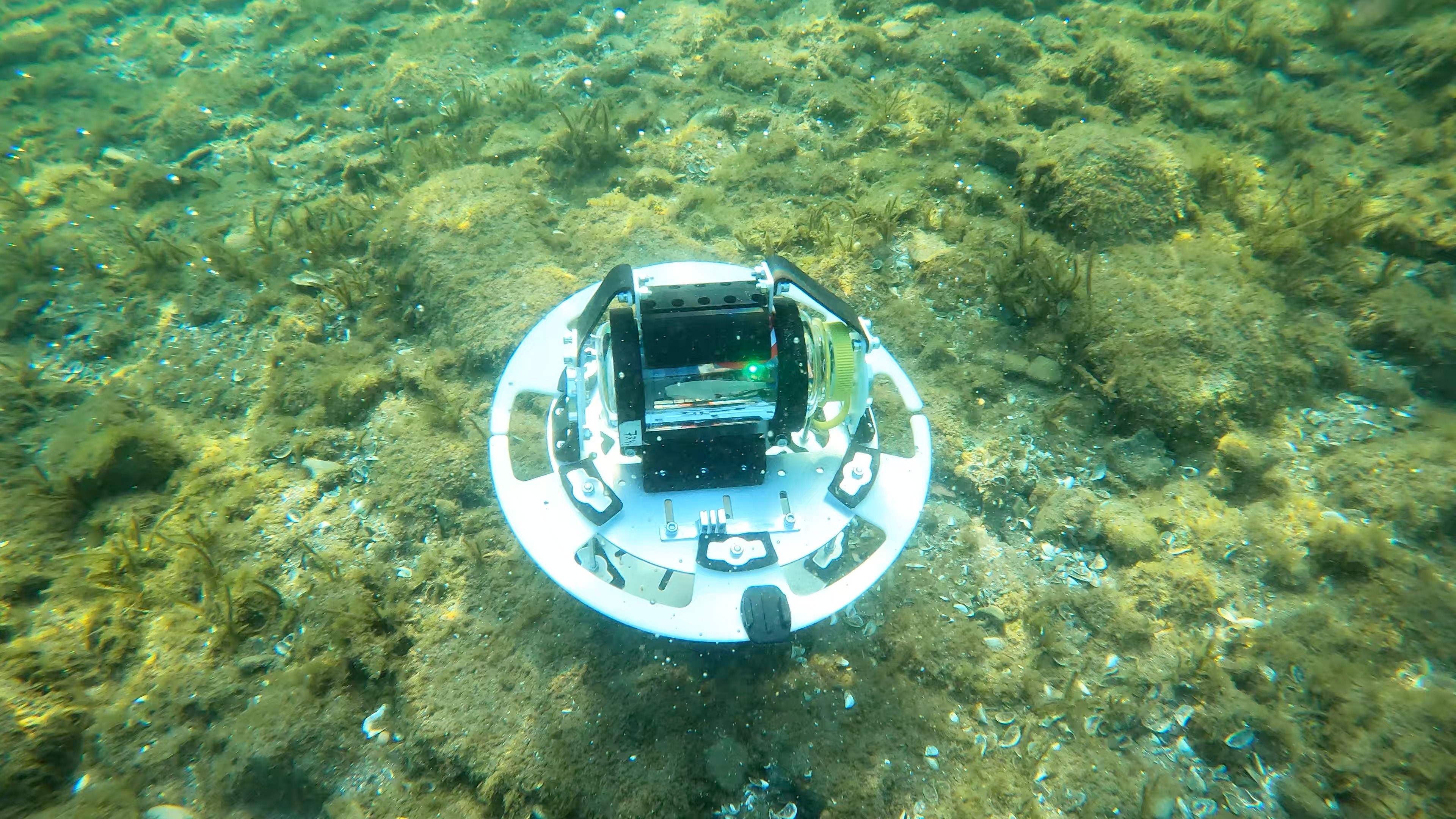
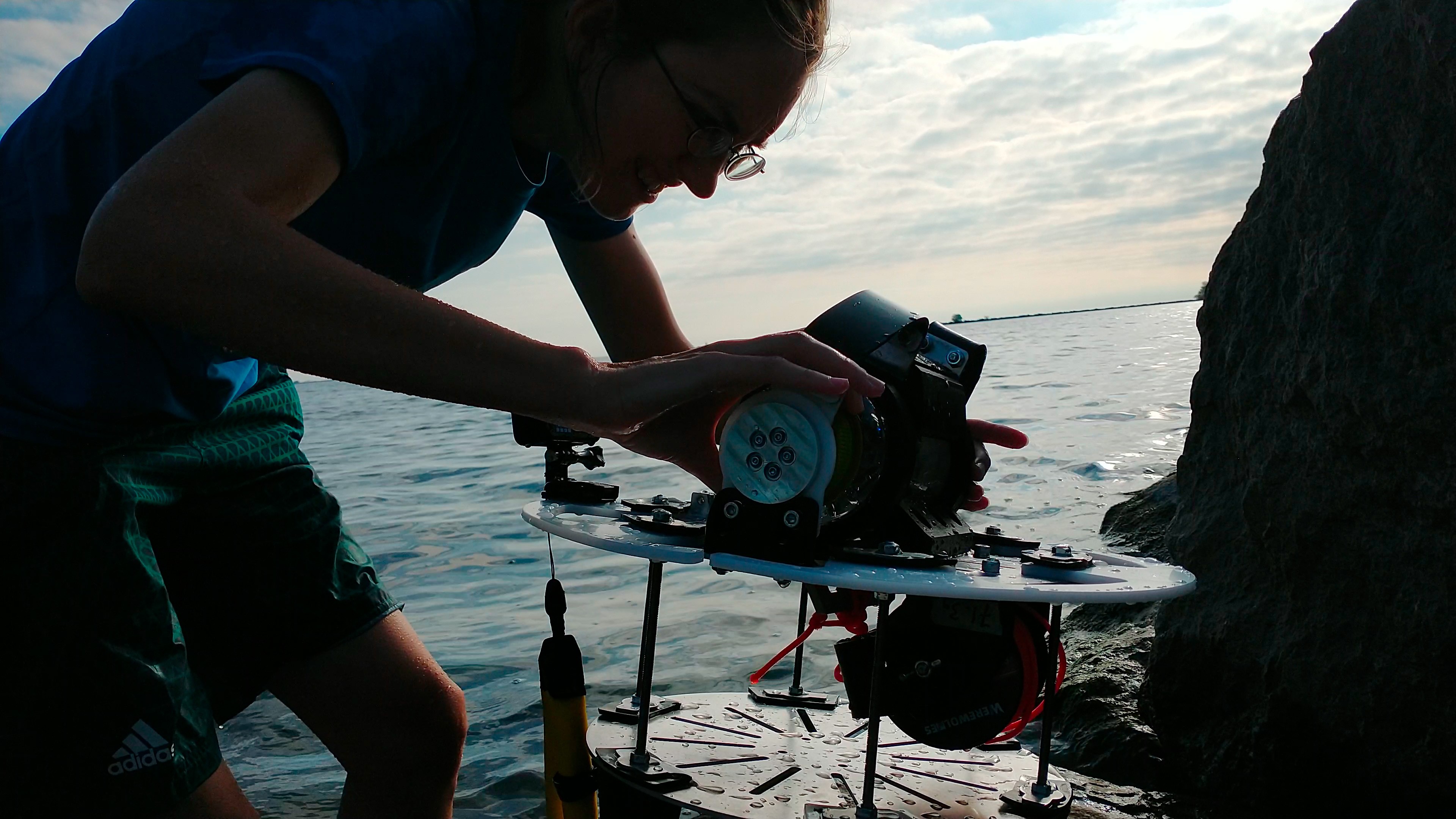
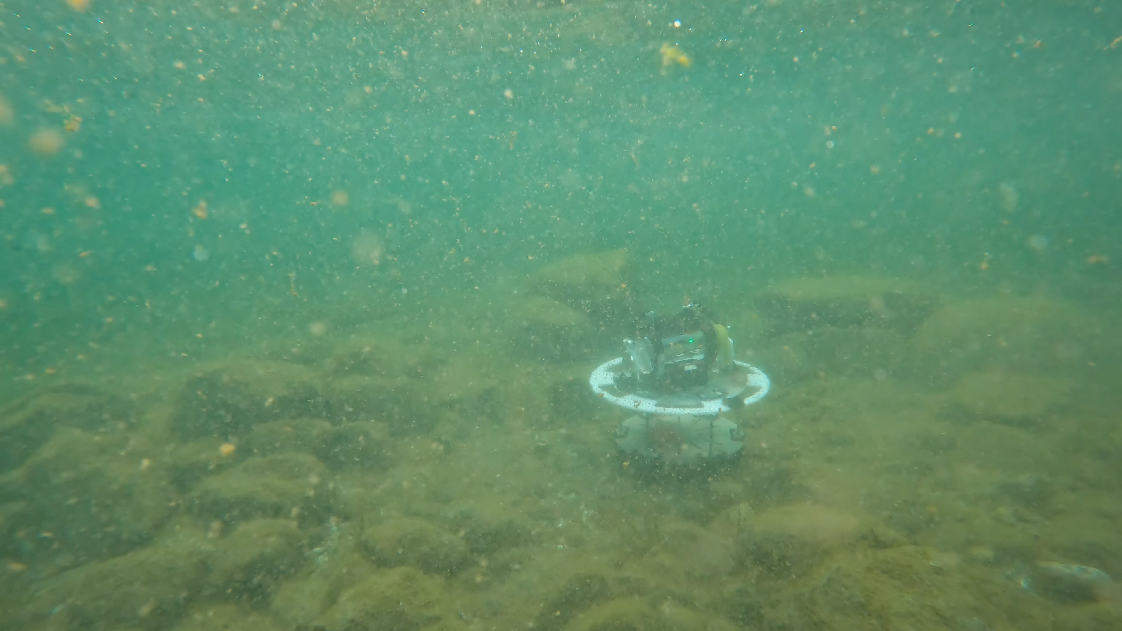
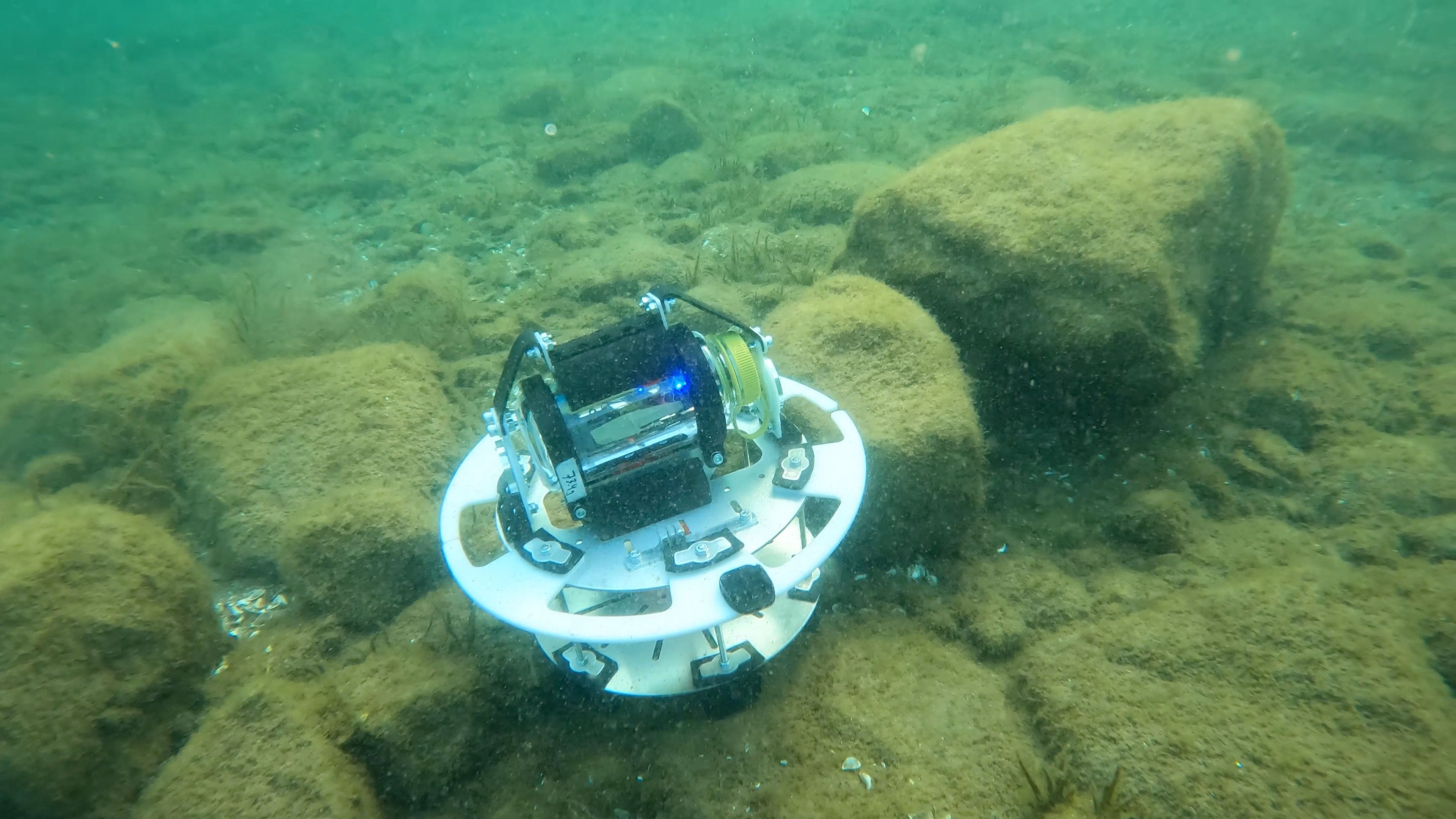
Field Test Photos
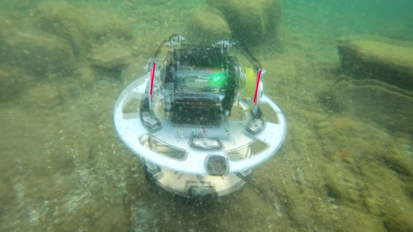
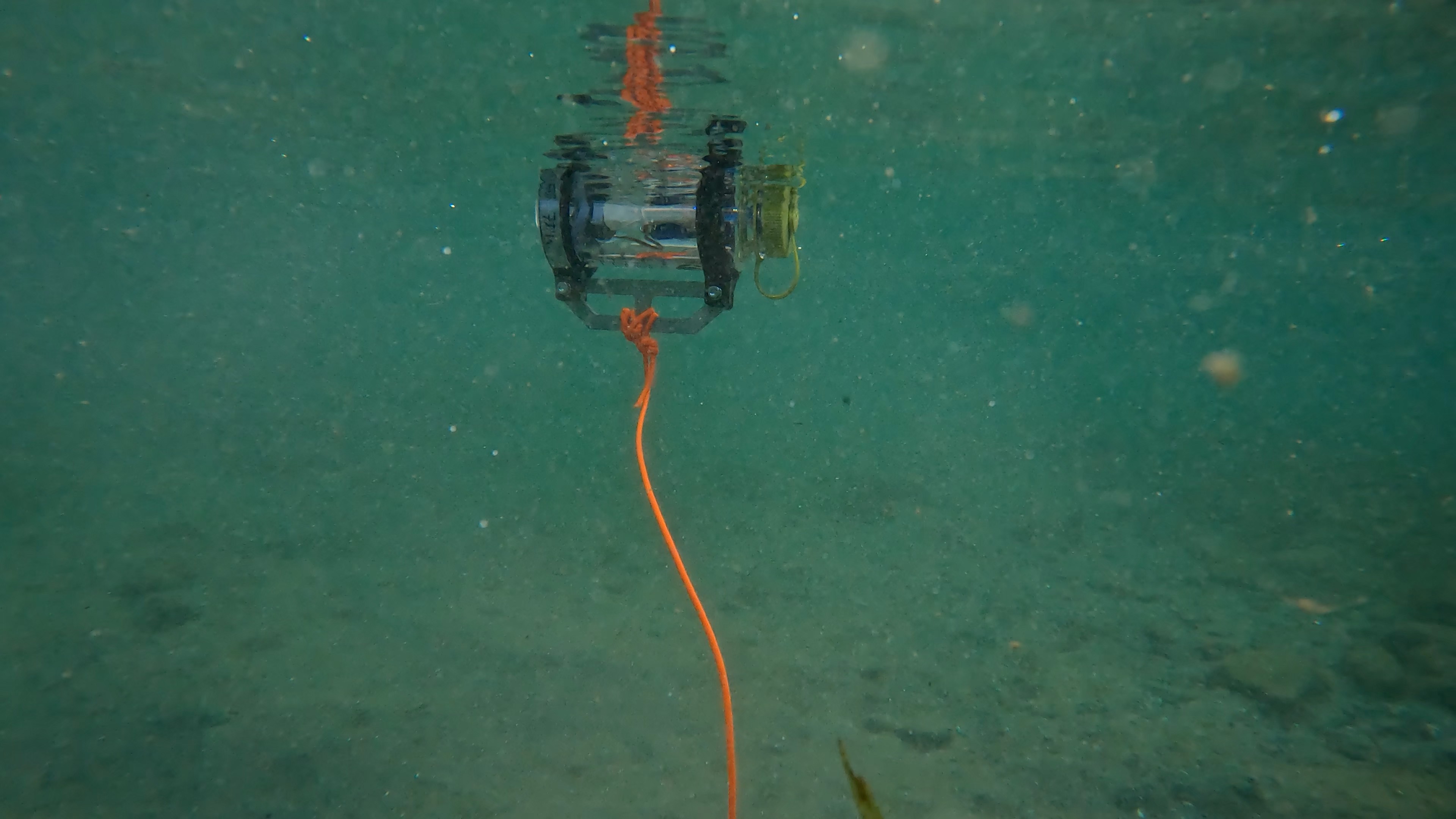
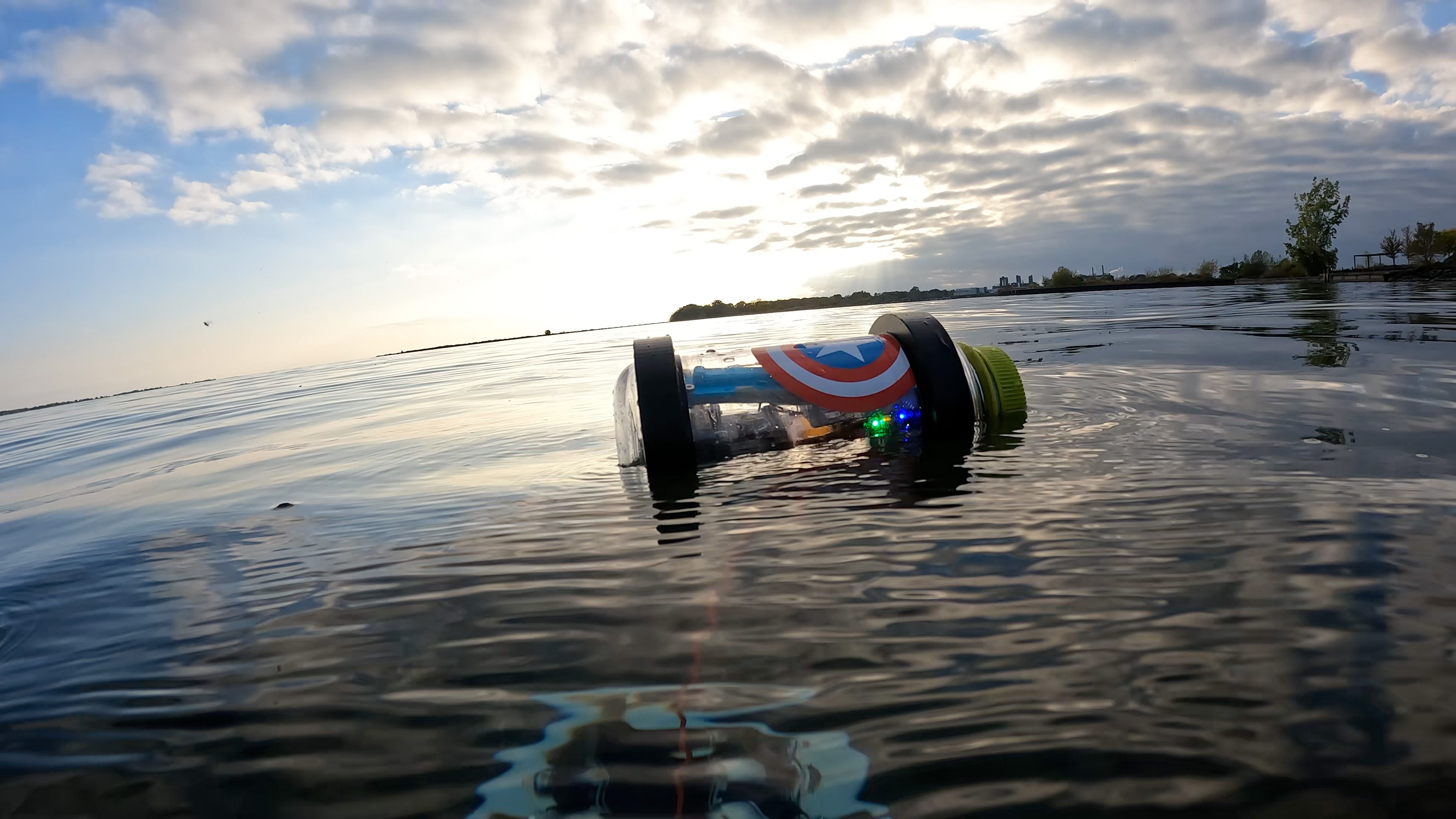
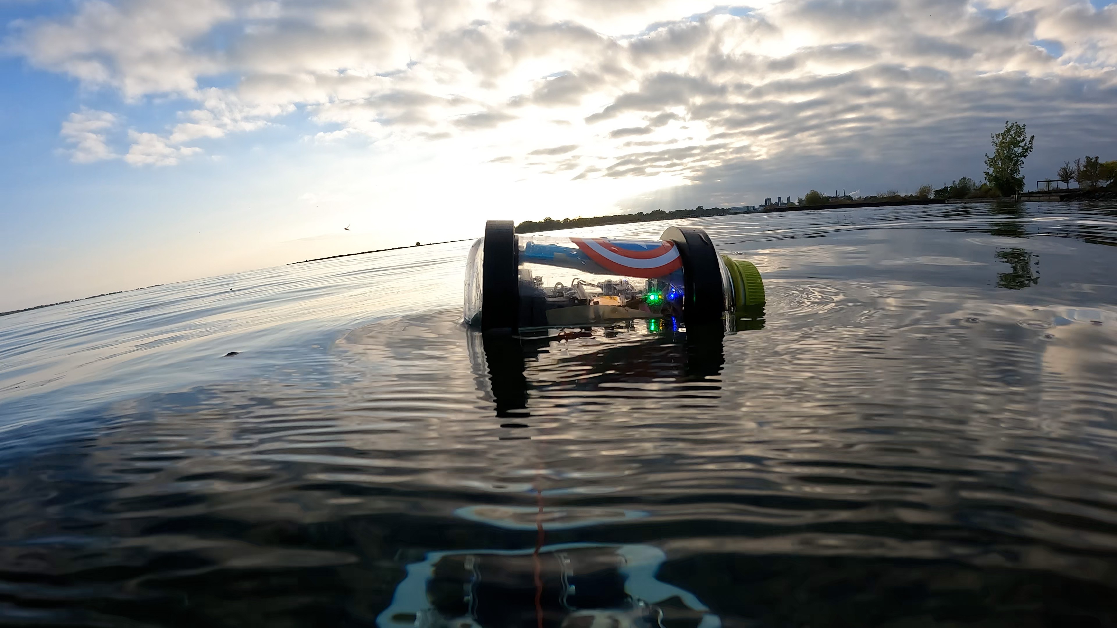
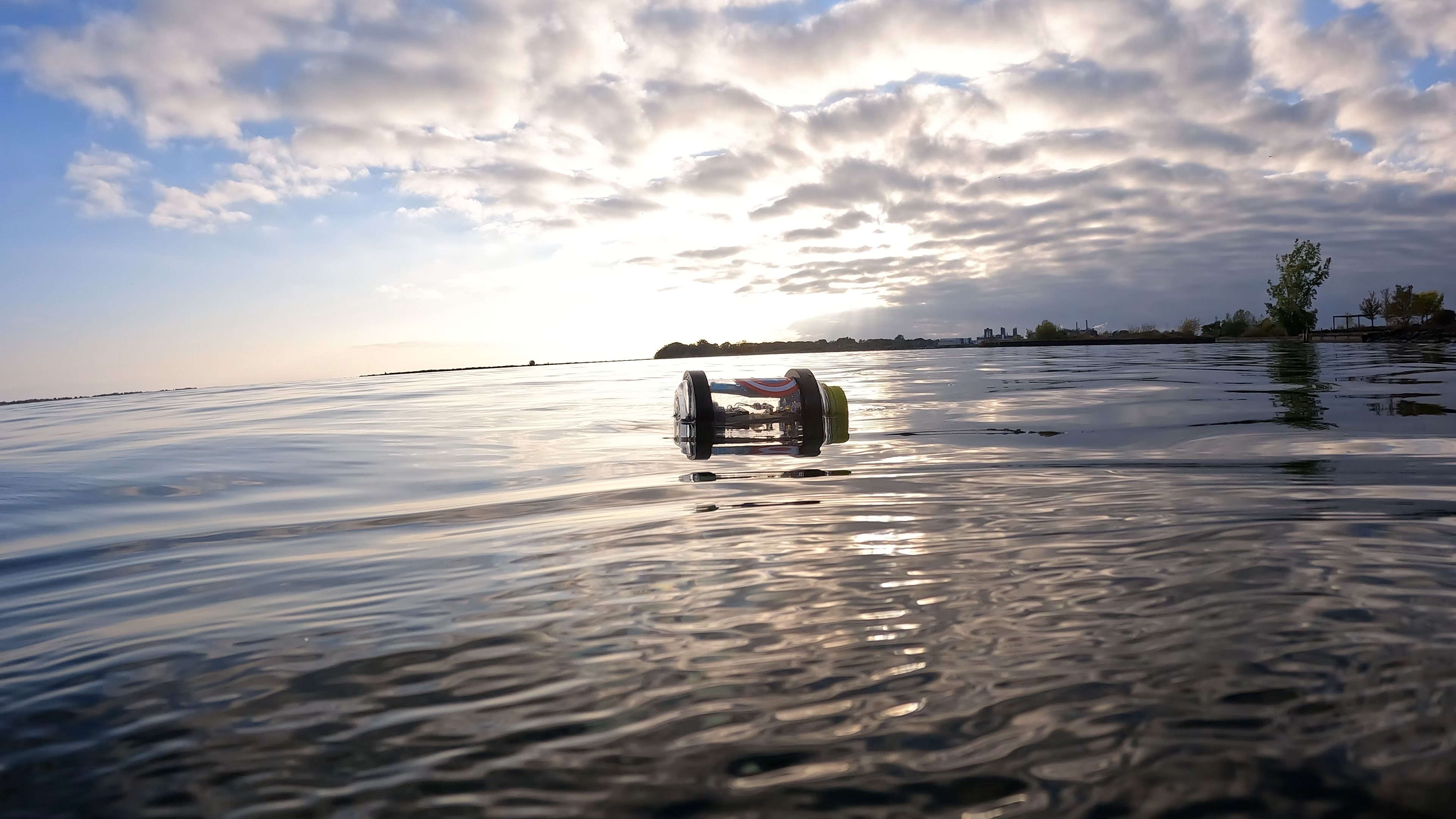
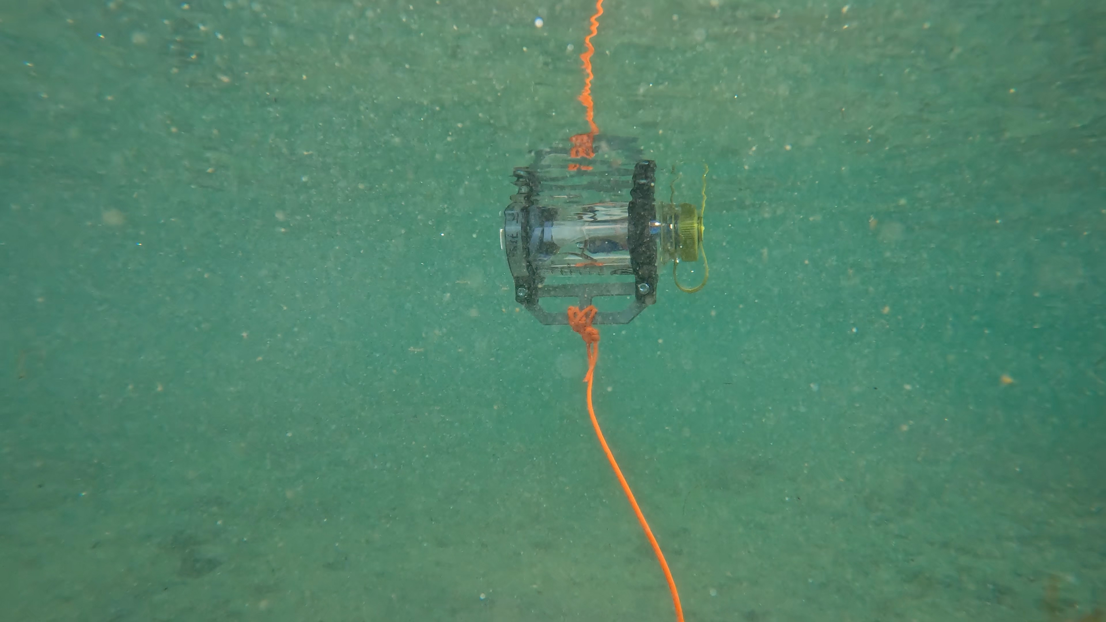
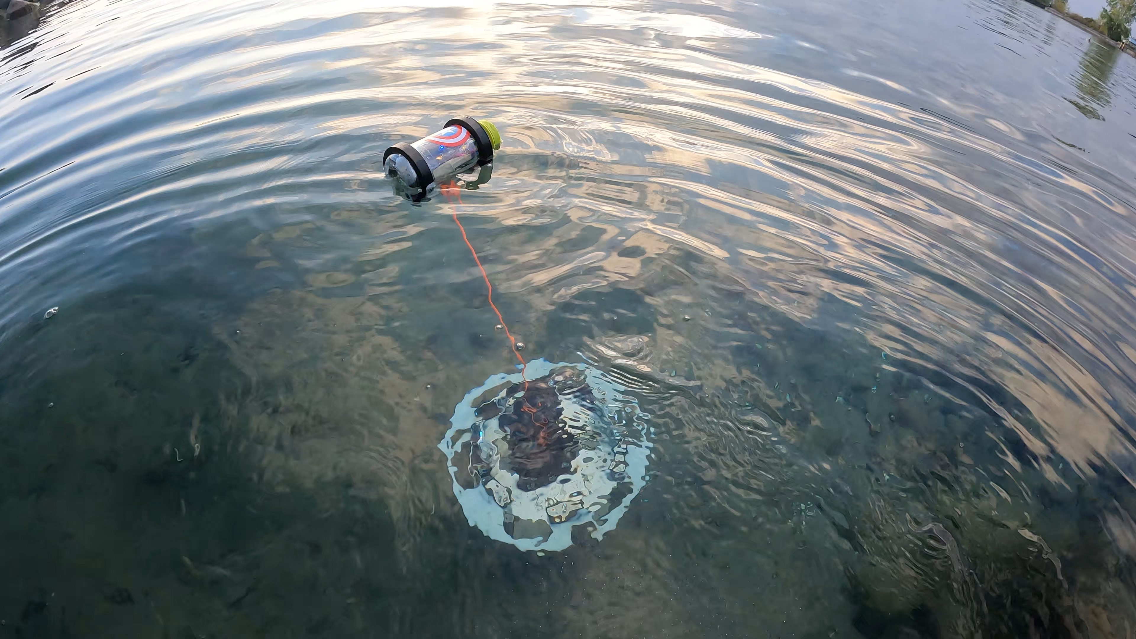
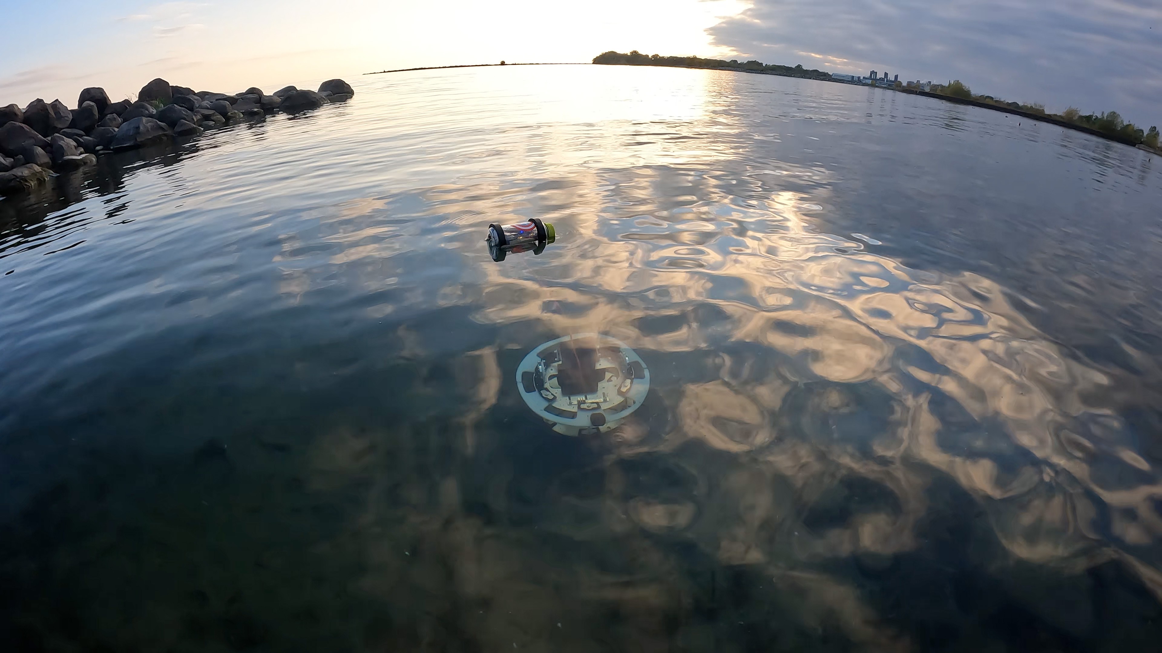
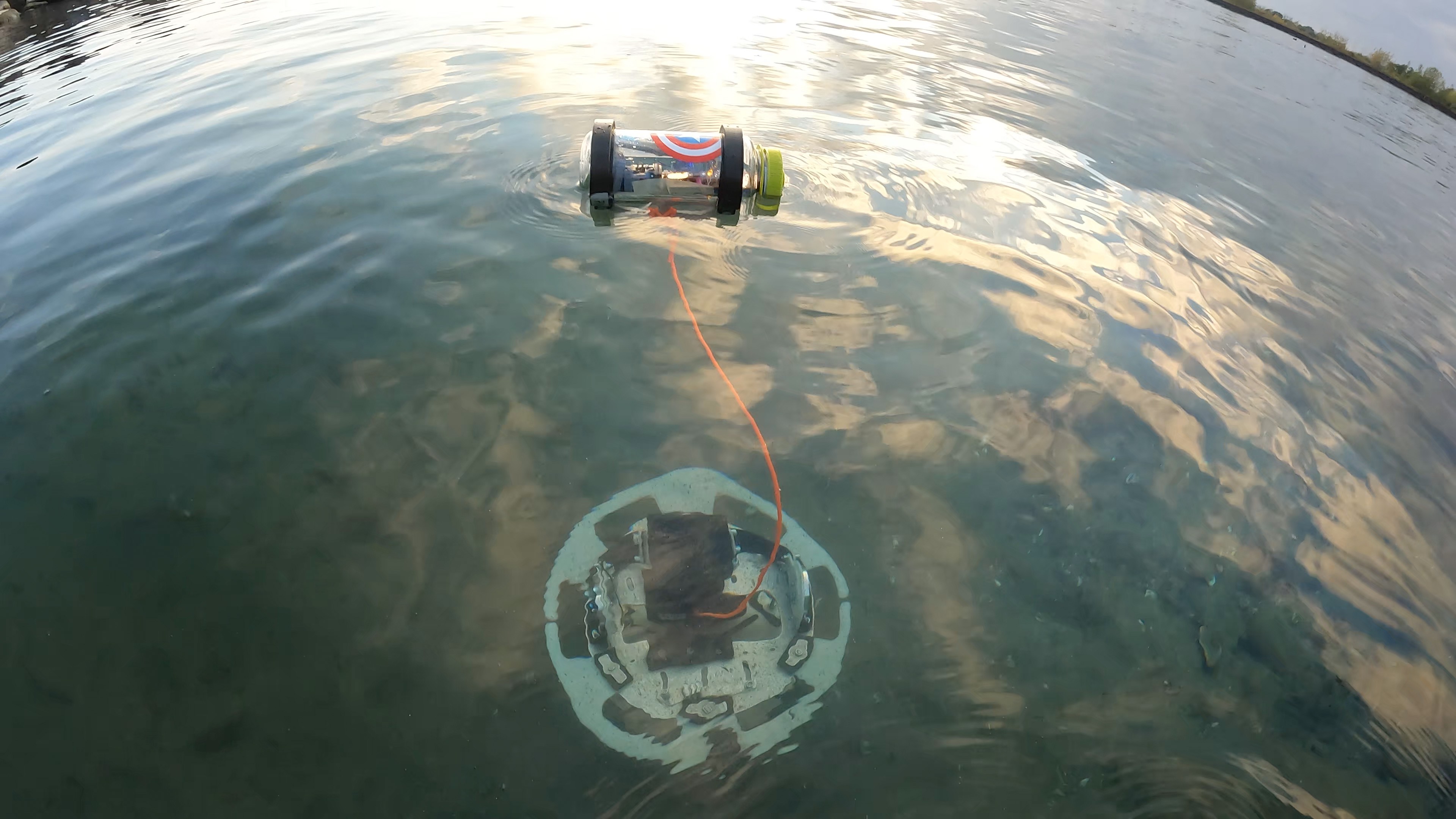
11/02/2021 at 03:13 • 0 commentsThe Field Test was a memorable moment - all of the work coming together at the deadline to test the robot. The sight of robots in the outdoors amongst nature is beautiful, knowing that these devices will help us better understand the environment around us. This is really the time of the project that’s very rewarding! Here are the top photos from the Field Test! Enjoy!!
![]()
![]()
![]()
![]()
![]()
![]()
![]()
![]()
![]()
![]()
![]()
![]()
![]()
![]()
![]()
![]()
![]()
![]()
![]()
![]()
![]()
![]()
![]()
![]()
![]()
![]()
![]()
![]()
![]()
![]()
-
Design Sketches
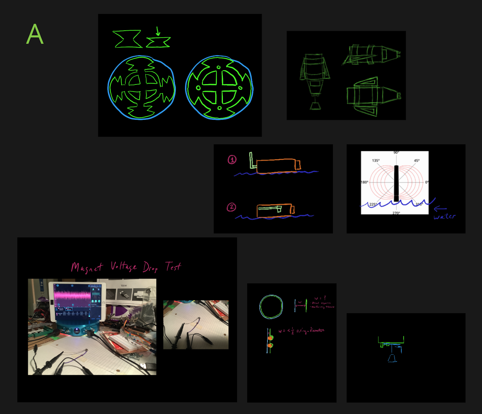
11/02/2021 at 02:57 • 1 commentAlong the way several concepts and areas for redesign were explored. This time, most of the sketches were done digitally. Here is a mosaic of all the sketches!
There were different stages during sketching. Here’s a summary collecting some of the thoughts.A: The beginning, getting oriented (see the buoy with different antenna orientations). Different ideas.
B: The somewhat finalized concept idea. This one had too many moving parts though. The commonality is the stacked stages.
C: Wiper magnets being closer and with less friction with a thin delrin sheet. This idea was later scrapped since Giovanni came up with a great solution - two low-profile ‘rails’ that the wiper glides on - reducing scratches, minimizing contact area, and less materials!
D: A lot of other ropeless fishing system designs use rope bags. What if there was a way to coil the rope? If it’s conical shaped, this would reduce tangling when coiling… however, if it is conical shaped, this means that the loading and landing orientation is 180 degrees flipped. This idea was scrapped because the centre of mass was at the top (for landing state, if it would even land like that).
E: Here was another concept. It is a tube cut in half with latch clamps. This idea just didn’t work logistically, and it seems like it would be cumbersome to try to reload the spool afterwards.
F: This is pretty well the final design, however the external enclosure (yellow lines) was excluded.
G: At the top right is the concept for the external wiper sub-assembly. The sketch in the middle played with an idea where there would be “flappy wings” on the side to help protect the buoy from waves. This wasn’t needed…
H: Does this look familiar?! It’s the concept for the stacks! Including some dampening foam (pink) on the threaded rods (yellow). This concept shows that the design is modular in terms of adding more stages to the stack
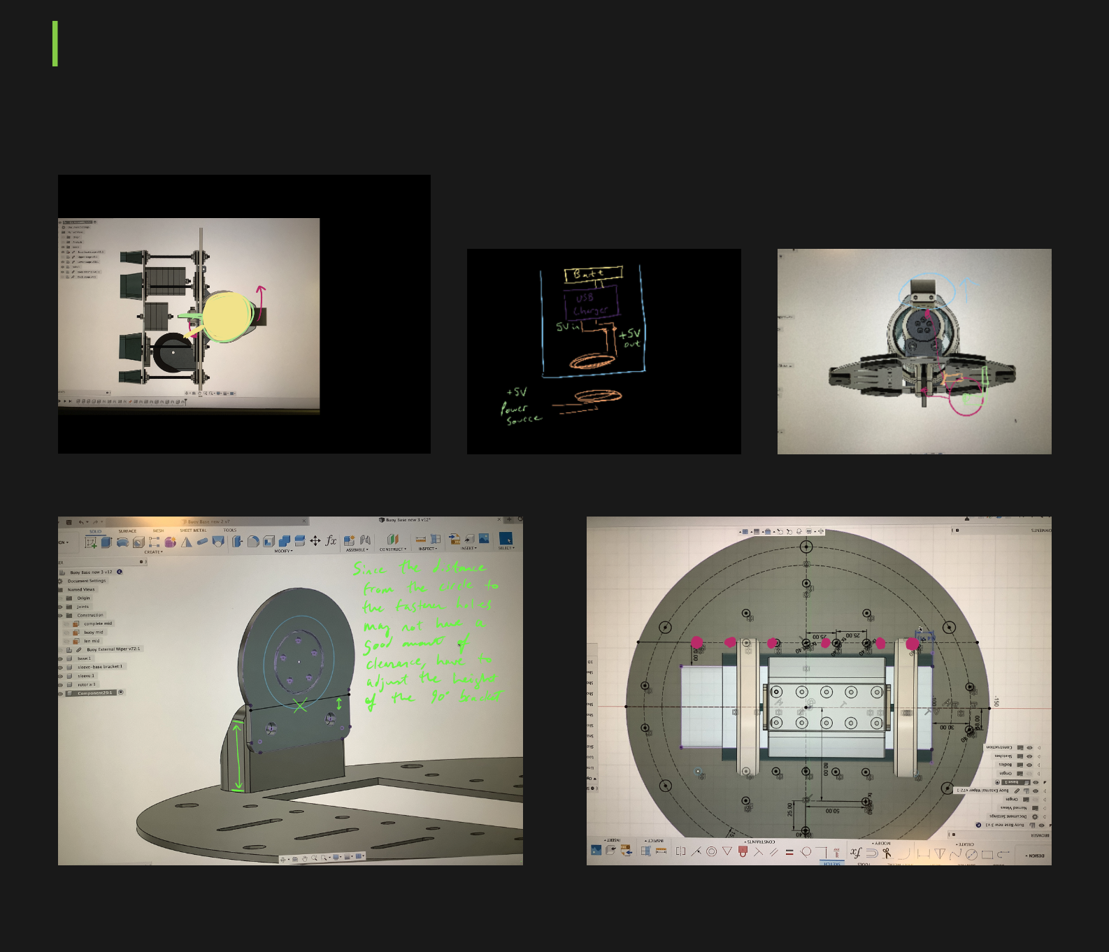
I: In between this sketch and the last one, CAD had commenced. As well, top middle, showing an idea for inductive charging - where the coil would be located. The sketch that was extremely useful was the one in the bottom right - for figuring out the spacing of the mounting holes for the buoy holder.
J: Electronics integration review with Leo! This was a great way to point out areas of concern on the integration side.
K: Uhh… we need a power switch, right? This is slightly difficult when using a sealed enclosure. This was an idea using a magnet and ball bearing to make contact on an internal switch piece. It’s based on the FINDA probe on Prusa printers.
L: These were sketches for the documentation of the physics model!
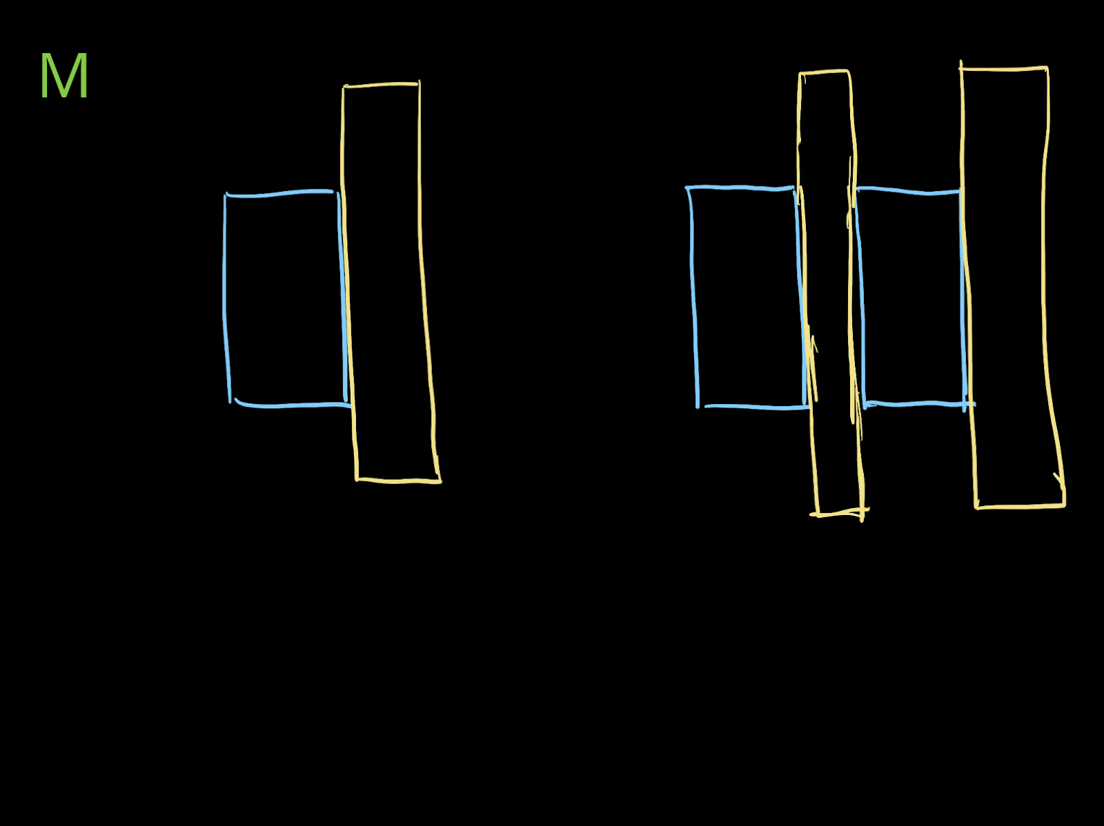
M: We will end on a funny note. This doesn't fit in with any of the groupings because... what on earth is this sketch? No clue! Let’s call it abstract art. :)
It was fun to look back on all the concepts and sketches through the project. Drawing is a very useful communication device! And hopefully this shows that it is not necessary to be a renowned artist to get started drawing.
-
Analysis of Field Test
10/30/2021 at 19:08 • 0 commentsThere is a possible failure that could occur with the delrin pieces of the sleeve bearing. On landing, these pieces deformed quite a bit:
Based on the observation above of the delrin deforming, knowing the force of the landing could better inform the parameters for simulation. To calculate this, the velocity of the descent needs to be determined.Descent Velocity
Observations from the descent of the robot can approximate the descent velocity in the water. A clip of the descent where the camera was somewhat stationary was chosen.
Between these two frames that are 2 seconds apart, we can see that the distance of travel is approximately 1 stand-piece-height. Each stand piece is 47.70 mm.
This means the robot travelled 4.77 cm in 2 s.v = Δd / Δt
4.77 cm / 2 s
= 0.02385 m/s
The descent velocity is 0.02385 m/s.
Force of Landing
When landing the robot immediately stops to 0 m/s. For “immediately”, this will be approximated as 0.1 s.
a = Δv / Δt
0.02385 m/s / 0.1 s
= 0.2385 m / s^2
The acceleration is -0.2385 m/s^2. The mass is estimated to be 7.0 kg.
F = m*a
7.0 kg * -0.2385 m/s^2
= -1.67 N
Or, -4.44 lbf.
It is important to notice that in the video there was a rock on the seafloor protruding higher than the others. This meant all of the force was on 1 of the 6 stands for landing. Usually, this force would be distributed over multiple stand pieces.
An attempt was made to simulate the force using a FEA simulation in Fusion 360 with the hope of determining the amount of displacement of the delrin pieces. However, this was not able to be completed in a timely manner due to additional configuration that would be needed on the simulation.
Ascent Velocity
Although the ascent speed is not needed, it would be interesting to know while we’re at it.
Using the same process as above, two frames from a video where the camera is almost stationary were extracted:
Overlaying the two frames, using the height of the buoy, the distance can be calculated:
Tracking from the bottom point of the buoy enclosure, the distance travelled is 4.3 buoy-body-lengths. Each buoy body length (aka diameter) is 92.64 mm.Total distance travelled = 39.8 cm.
v = Δd / Δt
39.8 cm / 2 s
= 0.199 m/s
The buoy ascends at 0.2 m/s. To travel the full length of the spool (30 m), it would take 150 s, or 2.5 mins.
Conclusion
To address the main issue at hand here about the delrin piece, two improvements are recommended:
- Add cushioning to the bottom of the stands (closed-cell foam)
- Increase material thickness of delrin pieces to 1/4"
Apart from that, more testing is needed to see where other parts break!
-
EJA - Improvements in the Electronics Design
10/20/2021 at 02:23 • 0 commentsSince the beginning of this project we have designed and tested different electronic designs, this log compares them and highlights their features, cost and dimensions.
We recently design EJA M v1.0 with the goal of replacing the previous designs, including some features (and removing the unused ones), reducing the cost and the size of the design. This log will show if the new design accomplishes those goals.
The project contains 2 different products (the Intelligent Buoy and the Onboard Gateway), each one has a different application, this log will compare the PCB designs that have the same application.
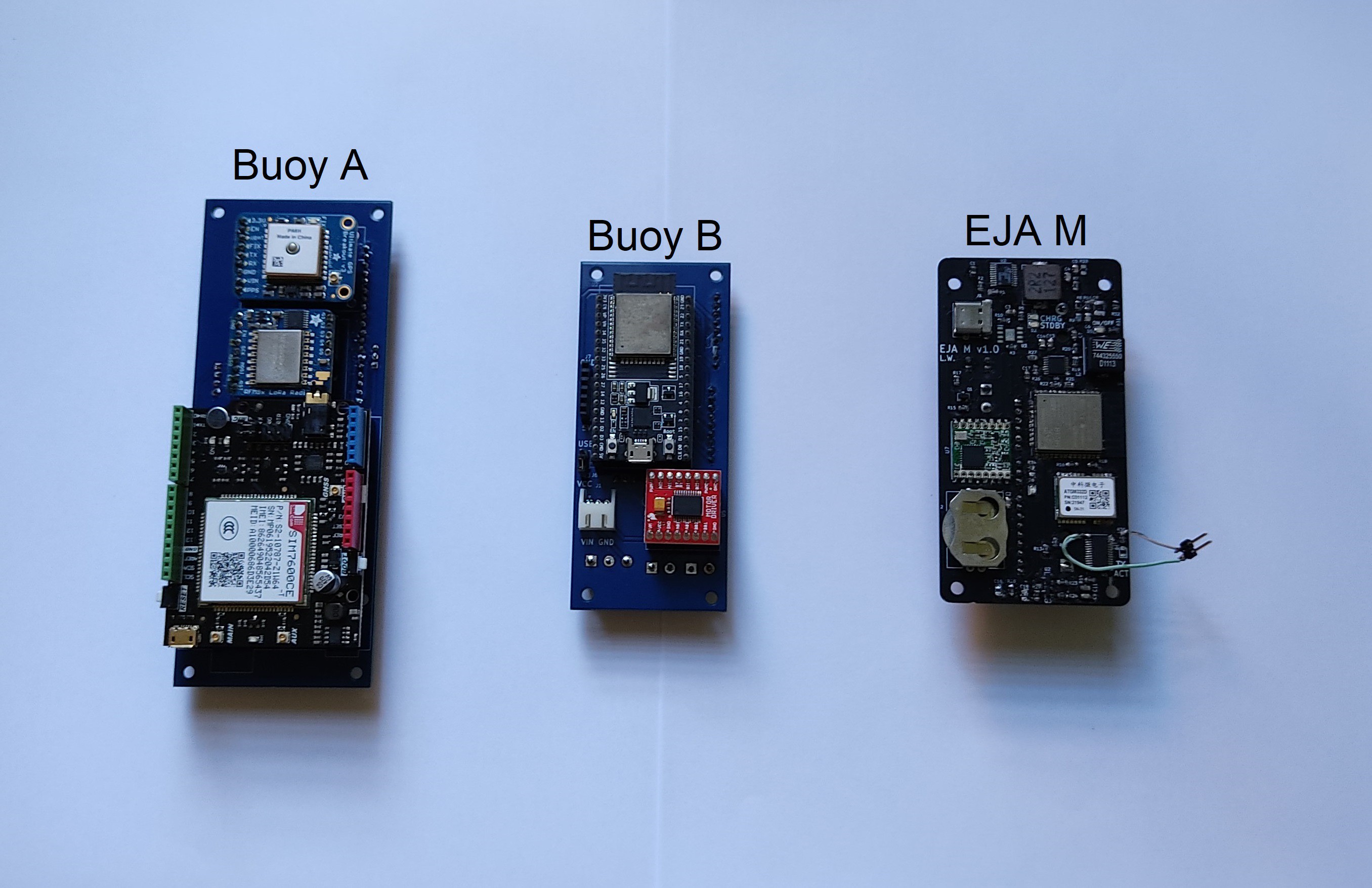
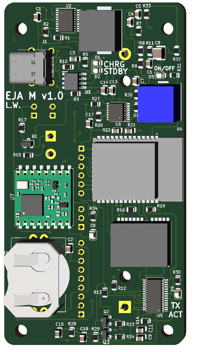
Intelligent Buoy
![]()
This device provides communication, a GPS for localization and activates the Ropeless System. To create an Intelligent Buoy we have designed 3 different PCBs in the last 2 years, those are:
Features
Those designs include the following features:Features Buoy A v1.0 Buoy B v1.0 EJA M v1.0 LoRa X X X GPS X X X Servo Motor X X X ESP32 X X X Real Time Clock X X X DC Motor X X 4G (LTE) X Battery Charger X Battery Level Indicator X Accelerometer X Cost
Buoy A v1.0 Buoy B v1.0 EJA M v1.0 $201.01 $131.02 $108.39 The following logs contain the detailed bill of materials of each design.
Size
Buoy A v1.0 Buoy B v1.0 EJA M v1.0 141.73 mm * 54.86 mm 102.36 mm * 44.2 mm 98 mm * 51 mm Notes: Buoy A v1.0 and Buoy B v1.0 require a 5V input, therefore they require a module or a PCB that provides 5V from the battery, this module will increase the required space for the design. EJA M v1.0 contains the power supply module inside the design, it can be connected directly to a 3.7V battery (or battery pack).
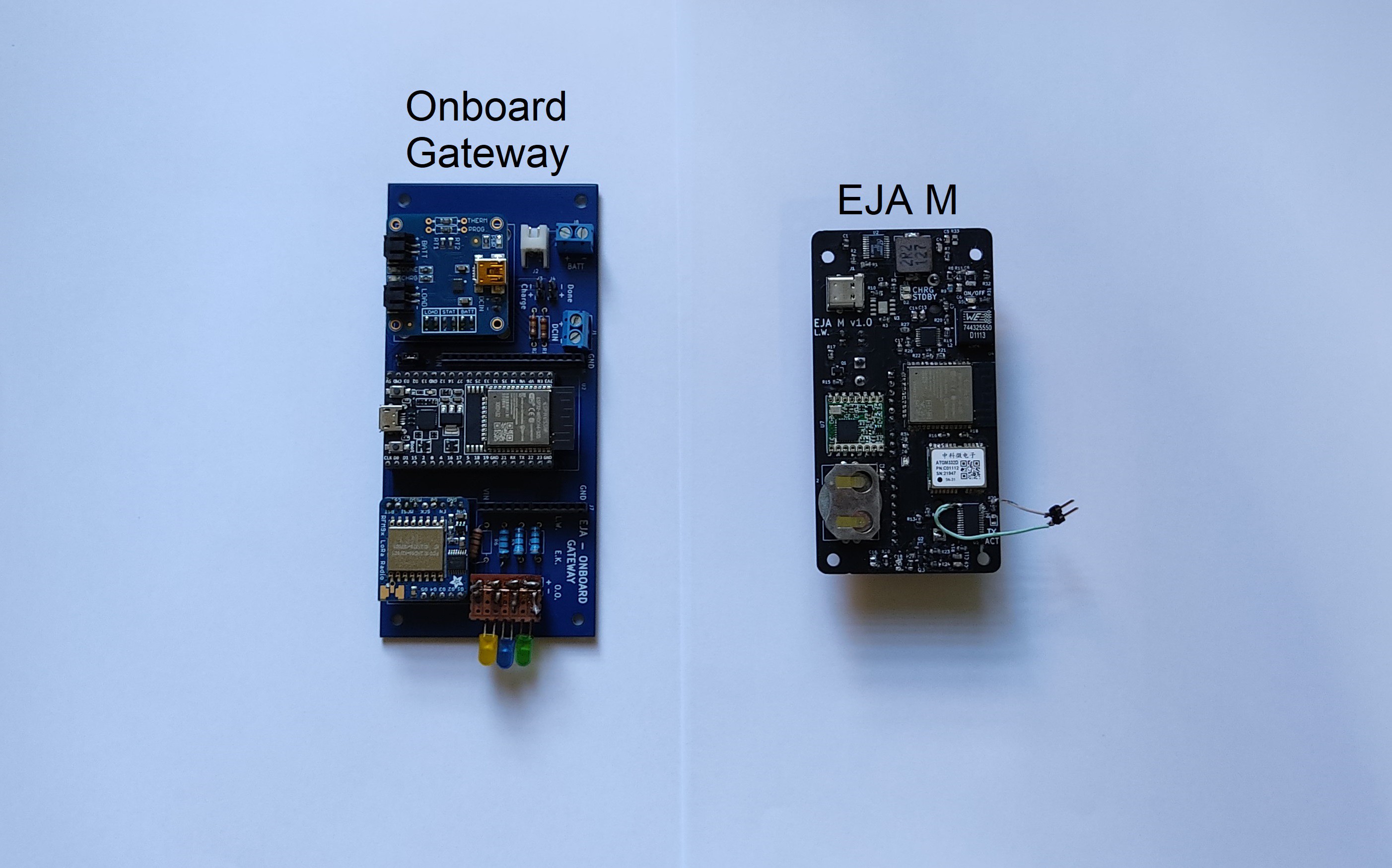
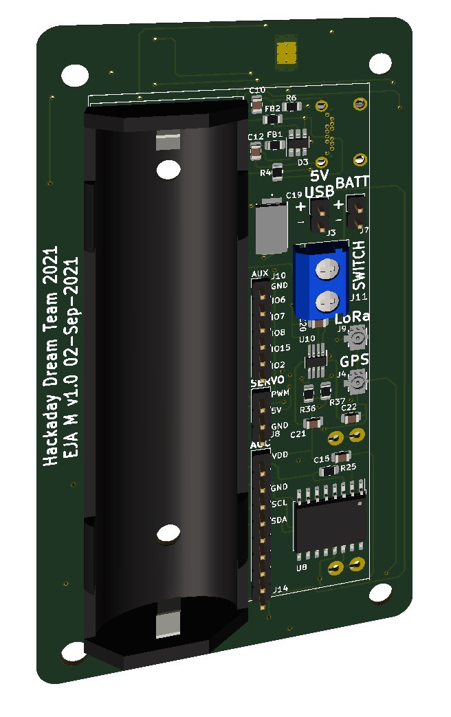
Onboard Gateway
![]()
This devices allows the user to communicate with the intelligent buoys. To create an Onboard Gateway we have designed 2 different PCBs in the last 2 years, those are:
Features
Those designs include the following features:
Features Onboard Gateway v1.0 EJA M v1.0 (Reduced Version) LoRa X X ESP32 X X Battery Charger X X Real Time Clock X Battery Level Indicator X The design EJA M v1.0 contains several features that are not present in the previous table, but they are not relevant for this application. In this comparison we are considering a reduce version of EJA M v1.0, it is basically the same PCB without the components that are not relevant in the application.
Cost
Onboard Gateway v1.0 EJA M v1.0 (Reduced Version) $84.34 $76.07 The following logs contain the detailed bill of materials of each design.
Size
Onboard Gateway v1.0 EJA M v1.0 (Reduced Version) 62.48 mm * 134.11 mm 98mm * 51 mm Conclusion
For both applications, we can conclude that EJA M v1.0 is a better solution considering the metrics that have been presented in this log: features, cost and size.
-
FTDI Development Board - Testing the Auto Reset and the FT260S
10/16/2021 at 16:13 • 0 comments![]()
This log includes the results of the tests made with the FTDI Development Board so far.
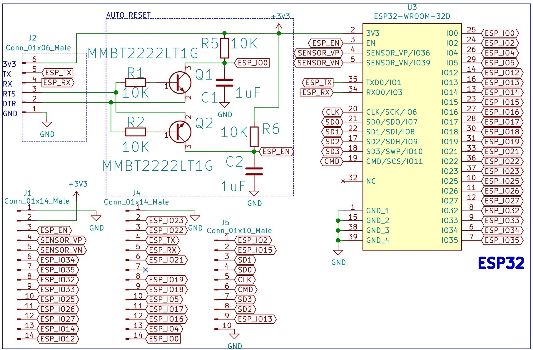
Auto Reset Circuit for the ESP32
The designed auto reset circuit requires the signals 3.3V, GND, TX, RX, RTS and DTR.
![]()
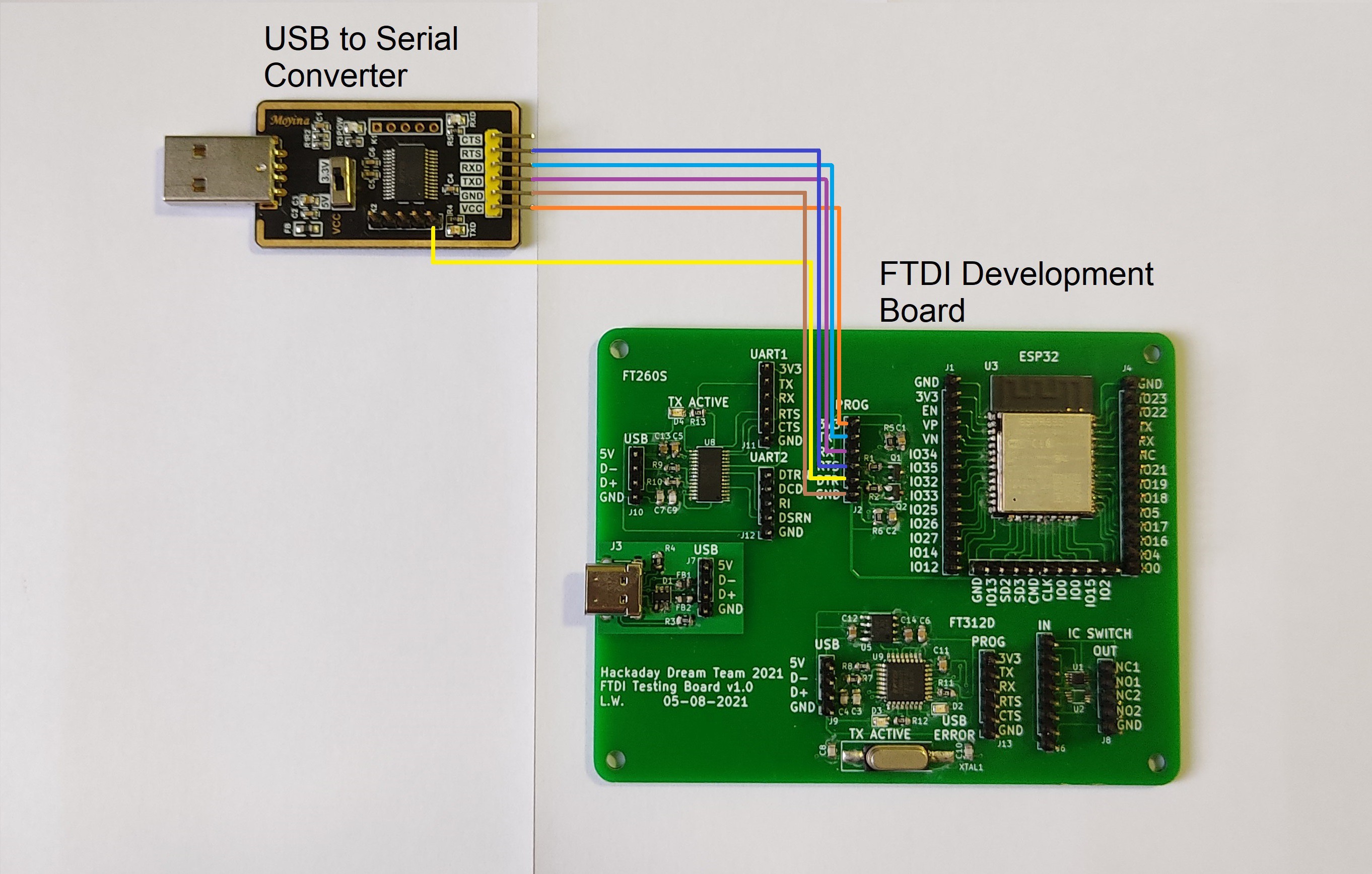
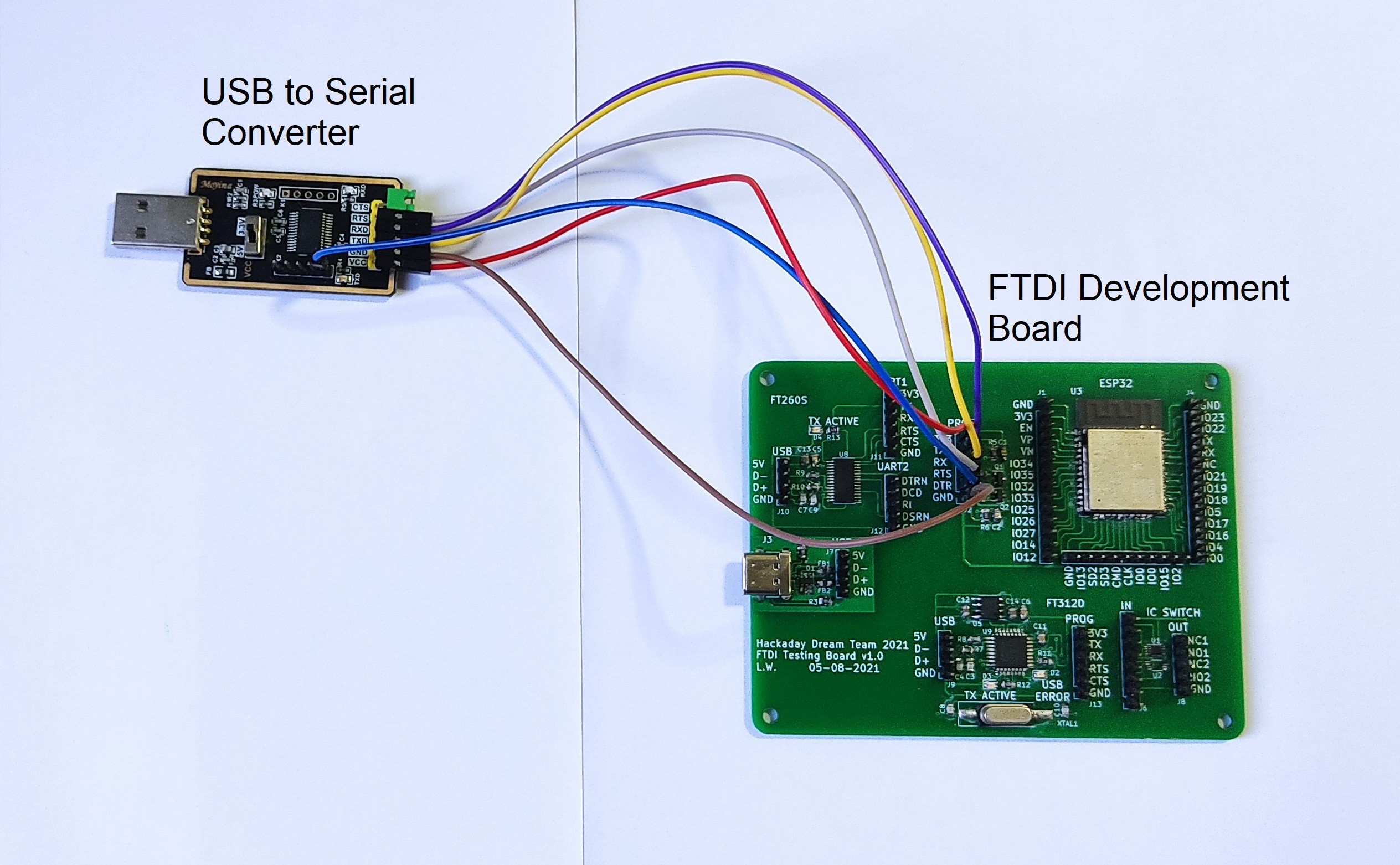
To test the circuit we used a commercial USB to Serial Converter that contains the FT232RL, and provides all the required signal.
![]()
The following wiring diagram shows how to connect the commercial USB to Serial Converter and our FTDI Development Board.
![]()
![]()
Once the 2 boards were connected and the USB to Serial Converter was plugged, the PC (in Windows) recognized the device and it was ready to use. Check if you need to install drivers associated to the FTDI, that is often the case.
Note: Before testing the following code, verify that the ESP-IDF is installed and the Arduino IDE can program ESP devices.
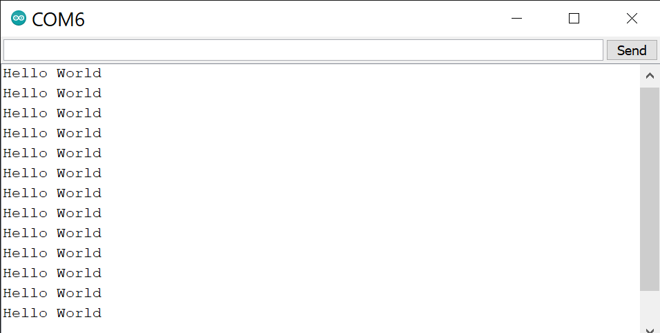
The code used is very simple, the ESP32 sends a "Hello world" message through the serial communication every second.
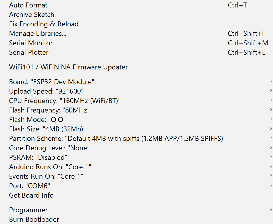
void setup() {
   Serial.begin(115200);
}

void loop() {
   Serial.println("Hello World");
   delay(1000);
}
To program the ESP32 we used the standard Arduino IDE, with the following configurations:
![]()
And the test was successful, the following image shows the results in the serial monitor.
![]()
FT260S-U
The FT260S was originally selected to directly program the ESP32, and also provide serial communication. After careful consideration I found that the FT260 is a HID class device and as such it does not generate a Virtual COM Port (like the FT232R), to interface with the FT260 it can be used the official helper library, LibFT260.
https://www.ftdichip.com/Support/Documents/AppNotes/AN_394_User_Guide_for_FT260.pdf
https://www.ftdichip.com/Support/Documents/AppNotes/AN_395_User_Guide_for_LibFT260.pdfFor that reason the FT260S will require more research before we can seamlessly program the ESP32. Sadly, this IC was selected for the newer design before realizing this information, so this topic will have to be addressed in the future.
-
Commencing Assembly!
10/04/2021 at 14:24 • 0 commentsAssembly is underway! Check out the videos showing the highlights so far from Day 1 & 2!
-
EJA M v1.0 - Bill of Materials
09/24/2021 at 15:51 • 0 commentsThis log presents the bill of materials of our new PCB EJA M v1.0. This new PCB will replace our intelligent buoy (Buoy A v1.0 and Buoy B v1.0), and our Onboard Gateway v1.0.
Full Version
To create an intelligent buoy we need to solder the complete PCB EJA M v1.0. The following table contains all the components and their current price (obtained at the moment of writing this log, it might change in the future).
PCB Components
External Components
Name Quantity Price SERVOMOTOR RC 5V HIGH TORQUE 1 $9.95 CR2032 Lithium Coin Cell Battery 1 $0.95 18650 Lithium-Ion 3.7V Battery Rechargeable 3.4Ah 1 $11.99 ADXL343 - Triple-Axis Accelerometer 1 $5.95 The overall price of the full PCB is $108.39.
Comparing the price to our previous PCB designs we have:
Design Buoy A v1.0 Buoy B v1.0 EJA M v1.0 (Full) Features - ESP32
- LoRa
- GPS
- Servo Motor
- Real Time Clock
- DC Motor
- 4G (LTE)- ESP32
- LoRa
- GPS
- Servo Motor
- Real Time Clock
- DC Motor- ESP32
- LoRa
- GPS
- Servo Motor
- Real Time Clock
- Battery Charger
- Battery Level Indicator
- AccelerometerPrice $201.01 $131.02 $108.39 Reduced Version
To create an Onboard Gateway we can use the PCB EJA M v1.0 with less components than the full version. The following table contains the required components and their current price (obtained at the moment of writing this log, it might change in the future).
PCB Components
External Components
Name Quantity Price CR2032 Lithium Coin Cell Battery 1 $0.95 18650 Lithium-Ion 3.7V Battery Rechargeable 3.4Ah 1 $11.99 The overall price of the full PCB is $76.07.
Comparing the price to our previous PCB design we have:
Design Onboard Gateway v1.0 EJA M v1.0 (Reduced) Features - ESP32
- LoRa
- Battery Charger- ESP32
- LoRa
- Battery Charger
- Real Time Clock
- Battery Level IndicatorPrice $84.34 $76.07 -
Physics Model
09/24/2021 at 15:49 • 0 commentsTo predict how our robot may perform in the real environment, a physics model would be useful to understand the forces at play. The calculated results serve as data points that can be verified experimentally to see how they differ in the real world.
---> EJA v2 Physics Model on Google Sheets <---
Highlights
Here's the key points from the calculations:
- In order for the weight to buoyancy ratio to be > 1.0, the mass of the entire robot has to be at least ~6 kg (13.2 lbs)
- Hydrostatic pressure at 30 m (100 ft) is 43.89 psi - roughly half of what we hypothesize as the limit for the Nalgene container
- At 50 m (164 ft), it is 73.16 psi, which would be an excellent test
- When the buoy reaches the surface, the tension on the line is 46.61 N, and the buoyancy-to-weight ratio is 1.25
- Based on the robot's total mass of 6.0 kg, with an initial velocity of 0 m/s:
- Terminal velocity is ~0.76 m/s, or 2.7 km/h (1.7 mph)
- Landing force is ~-8.5 N, or almost 2 lbf
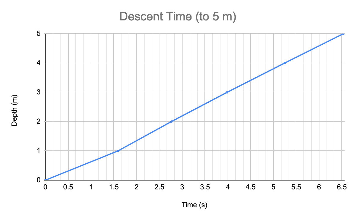
- To reach 5 m, it takes 6.5 seconds
- To reach 30 m, it takes 39.1 seconds
- If freefalling for 1 min, the robot would descend 46 m
- To reach 1000 m, it would take 21.7 minutes
- (At that point, the pressure at 1000 m is 1468.95 psi though!)
To improve the physics model calculations, we will verify experimentally:
- Mass
- Buoy
- Rope spool
- Entire robot
- Ballasts
- Percentage of buoy submerged when at the surface
- Descent time
There are scenarios of what we want to calculate:
- Buoyancy
- Terminal velocity
- Drag force
- Freefall velocity - Descent time to target depth
- Hydrostatic pressure
- Tension of the rope
Let's dive in to each scenario!
1. Buoyancy
The weight to buoyancy ratio is the key number to making sure the robot will sink.
Buoyancy is all about the volume of liquid displaced by the robot. This is why a steel boat can still float, yet a steel ball will sink - because of the volume. The density of the material does not matter.
The volume of the robot is estimated to be 4753 cm^3.
The minimum mass must be 6.0 kg to get the weight-to-buoyancy ratio to be > 1 (meaning, it will sink). For a mass of 6.0 kg, the weight-to-buoyancy ratio is 1.169.
The addition of ballasts was added in CAD to fine tune the position of the centre of mass. Further experimentation will need to be completed to ensure that it is the correct amount of ballasts to achieve 6.0 kg.
In CAD, we see the estimation of the mass to be 12 kg. However, skeptical of that number based on the real world materials. Actual mass will need to be confirmed experimentally when the robot is entirely constructed.
Thanks to Leo for the post from last year that breaks down the buoyancy topic very well!
2. Terminal velocity
A large terminal velocity could impact the robot by inducing vibrations when landing, having a risk of unseating the magnet wiper. As well, imprinting the seafloor. Minimizing this would reduce those impacts.
Based on a mass of 6.0 kg and a target depth of 5 m,
The terminal velocity for the robot is 0.766 m/s. For comparison, that is ~70% of the typical human walking speed (2.5 mph).
Although there is no term for depth, the model does change as the density of water changes when going deeper. For seawater, the linear change in density was extrapolated from this table (Source: Encyclopedia Britannica). The scale of the change is very small: 0.01 m/s total difference from 0 m to 10,000 m depth.
The drag coefficient was selected to be 1.55. This is based on the inverted triangle shape, which the robot somewhat looks like given the diameter of the handles on the upper stage are larger than the diameter of the lower stage. (Source: Sighard Hoerner, Fluid Dynamic Drag via Wikipedia)
Another way of minimizing terminal velocity would be to streamline the design, thereby reducing the coefficient of drag and area.
3. Drag force
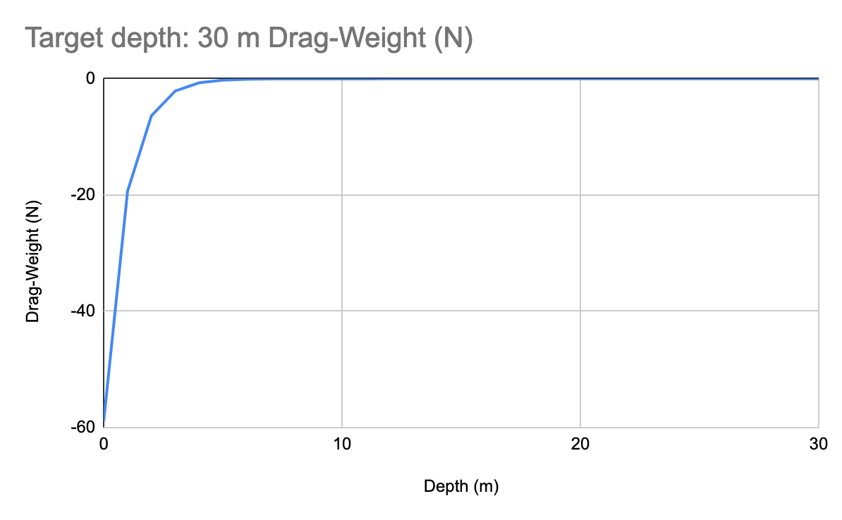
As the robot is descending through the water, there is a drag force pointing upwards against the robot.
What we expect to see is drag and weight balance out at some point. Sometimes this can happen before the target depth is reached. For this model, there is a drop-off around 5 m. This graph shows the difference between the drag force and weight. This approaches 0 as the forces balance out.
The freefall velocity is a term in the drag force equation that plays a role in this. This will be discussed in the next section.
Something that is concerning is a different scenario where the robot is entered in to the water at a 90 degree angle. Meaning, it's not pointed down, it's on its "side". The drag force will be different as the area will change along with the coefficient of drag.
Verifying experimentally the behaviour of the centre of mass will be useful in determining if more work is necessary for such edge cases. User feedback will be useful in seeing how often those edge cases happen in reality (perhaps they happen more often than not!).
4. Freefall velocity - Descent time to target depth
How much time the robot takes to reach the target depth depends on the freefall velocity. Freefall velocity is also a term that is used in the drag force formula.
Note: In the physics model, the square root is taken on the above formula to obtain the v value.
Assuming the robot starts with an initial velocity of 0 m/s,
To reach a depth of 30 m it will take 39.1 seconds. For shallow water testing of 5 m, it will take 6.5 seconds. To reach 1000 m, it would take 21.7 minutes. Wow!
The relationship appears linear for the most part because the depth where freefall velocity approaches terminal velocity is 2.88 m.
The non-linear relation is evident in the first 5 m (you have to look carefully around the 1.5 to 3 second mark, but in the numbers it is evident).
This is controlled by the exponential decay term in the formula for drag. In that, y represents the current depth. In our model, we used a ratio of current depth to target depth as y.
The formula for freefall velocity where the independent variable is distance is derived from freefall velocity as a function of time. The full derivation can be found on Hyperphysics here.
As mentioned in the previous section, the drag force balances out with the weight force after a portion of time, and that is controlled by the exponential decay term.
5. Hydrostatic pressure
Hydrostatic pressure increases with the depth. This is of importance since if the pressure is too much for the material, the buoy's Nalgene enclosure will be destructively compressed or shattered.
Our hypothesis is the current buoy enclosure might withstand ~80 psi (based on this video). This would set 50 m as the depth limit at 73.16 psi with the buoy in its current configuration. In the upcoming shallow water testing, it's predicted the pressure would be ~7 psi.
Depth (m)
Hydrostatic Pressure (psi)
5
7.31
30
43.89
50
73.16
100
146.35
1000
1468.95
10000
15238.97
Going from 50 m - 500 m, and onwards, a different enclosure strategy for the buoy will be needed.
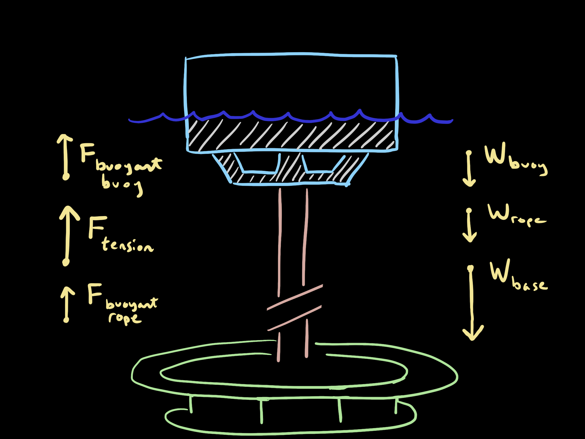
6. Tension of the rope
The rope is the vertical line that goes from the base on the seafloor to the buoy on the surface. If this rope is under a lot of tension, this also cuts into the whale when entangled and swimming. This is why some ropes have weak links or weak insertions, which break after a certain amount of force, so the whale won't be dragging the gear along with it.
The tension force points upwards, countering the weight of the buoy and rope. It is assumed that the buoy is submerged 50% when it is at the surface — which influences the volume calculation for buoyancy. The mass of the buoy and the mass of the rope is assumed to be 0.5 kg each (this is a wild estimate, and needs to be verified in reality).
Based on the robot mass of 6.0 kg, an entire spool of 30 m, and the buoy submerged by 50%:
The tension on the rope is 46.61 N, or 10.47 lbf.
That is approximately 1/16th the tension on a piano string.
While looking at these numbers, it would also be beneficial to see the buoyancy-to-weight ratio to ensure the buoy will float. The buoyancy-to-weight ratio is 1.25, meaning the buoy will float with this rope.
There are a lot of variables at play here where the model probably falls short. For example, fishers may use weighted line, and the diameter may be larger. There may be water currents that pull the buoy away from the base. Verifying experimentally will allow us to see the validity of these calculations.
Assumptions and errors
Some assumptions in this physics model are:
- Assumption about drag force only balancing out when reaching the target depth
- Using a ratio of depth/target depth in the exponential decay term for freefall velocity
- Miscalculations in volume (for example, if excluded bodies in the model were included when Fusion 360 calculates this — further investigation is necessary)
- Cross-sectional area for drag force (would this be an average of the lower stage and upper stage area? or the largest area?)
- Coefficient of drag was set at 1.55 based on a cone that is larger at the top (source)
- Extrapolated a linear formula of density of seawater for the various depths (source)
- Assuming the drag force balances out at the target depth, this would mean that the landing force would always be the net force
- Skeptical of the mass estimation in Fusion 360
As a flaw, this physics model addresses the "best case" scenario. Namely, when the robot is oriented in the proper direction and enters the water from rest. A next step could be to try to model what happens when the robot enters at a 90 degree angle, and when the robot is submerged with an initial velocity. Observations through trial and error in real world testing can help with adapting the model for those scenarios.
Conclusion & Next Steps
It has been an absolute blast to prepare this model, reviewing these concepts again. This gives some data points to compare the real world testing to. Eager to test to see how far off the results actually are.
Next steps are to test this in the real world and see how it performs, and adjust the model as necessary.
Any mistakes in here are my fault. Know something that could be better? Leave a comment below :)
-
RFM95W-915S2 Development Board - Testing
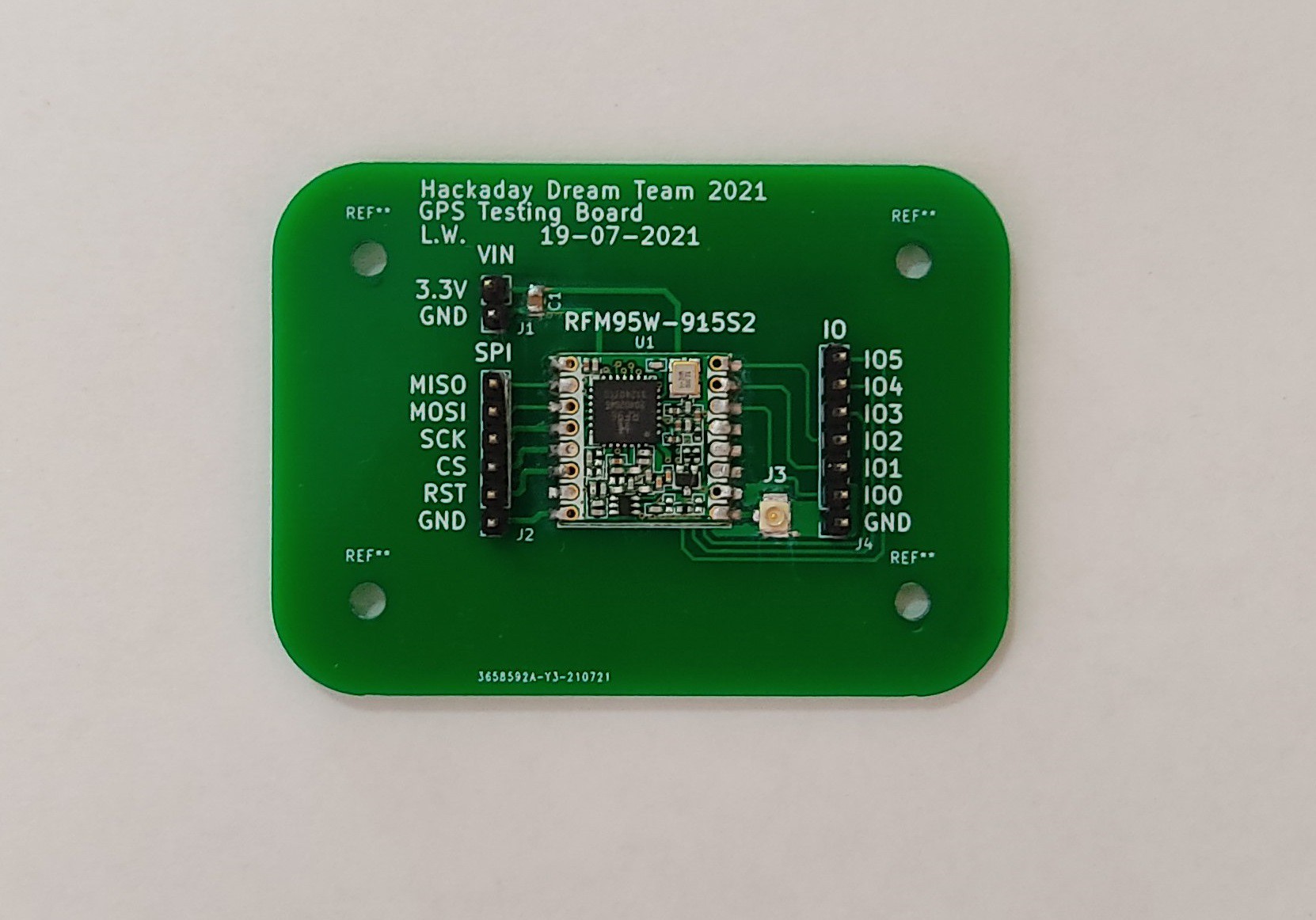
09/21/2021 at 20:29 • 0 comments![]()
The RFM95W-915S2 Development board is a PCB that contains a RFM95W LoRa transceiver, a U.FL connector for the external antenna, a decoupling capacitor and a group of headers connected to the different pins of the transceiver. The transceiver can be used as a sender or a receiver.
This log describes the initial tests that were performed using the RFM95W-915S2 Development board.
Wiring for the Tests
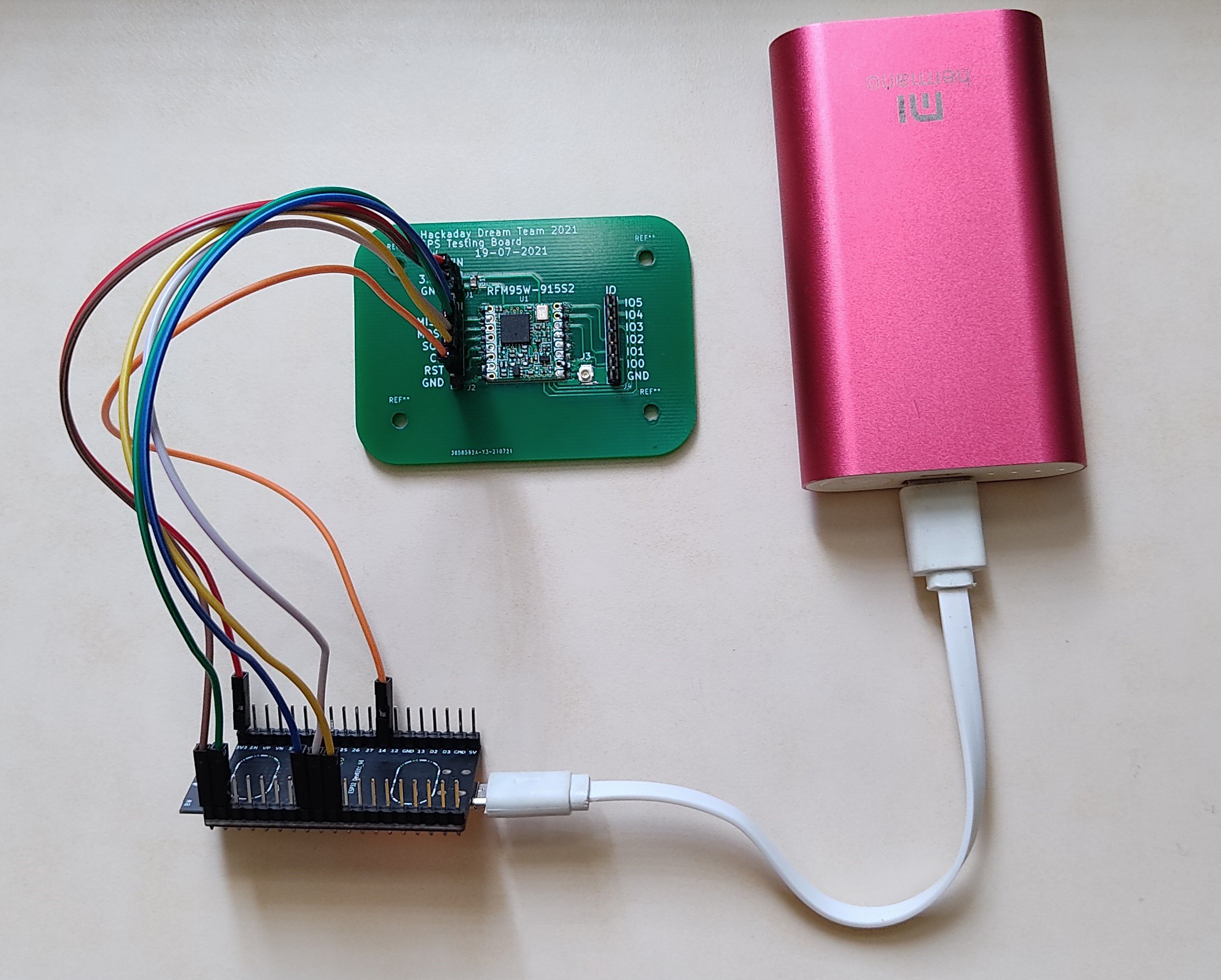
The webpage randomnerdtutorials.com has an amazing tutorial named ESP32 with LoRa using Arduino IDE – Getting Started, that tutorial contains detailed information about how to use the RFM95 with an ESP32 (the same microcontroller that was selected for our designs). I used the same firmware and connections provided by the tutorial.
The test requires 2 transceivers, one of them will be used as a sender and the other as a receiver. In this case, one of the transceivers is the RFM95W-915S2 Development board and the other one is the RFM95W transceiver from Adafruit.
The connections are the following:
ESP32 RFM95W-915S2 Development Board 3V3 3.3V GND GND GPIO 14 RST GPIO 5 CS GPIO 18 SCK GPIO 23 MOSI GPIO 19 MISO ![]()
ESP32 RFM95W Board from Adafruit 3V3 VIN GND GND GPIO 14 RST GPIO 5 CS GPIO 18 SCK GPIO 23 MOSI GPIO 19 MISO ![]()
Firmware
The firmware can be found in the following Github repository. The repository contains a folder named /Firmware/ that contains the project for the transceiver as a receiver and a sender.
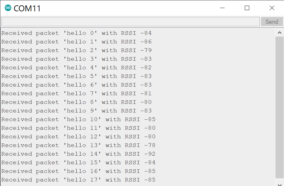
Both of the RFM95W Boards were used as a sender and receiver, the result was successful in both cases. During the test, one of the transceivers sends the package "hello counter", where the counter is a number that goes from 0 to 32767. The other transceiver receives the package and prints the message through serial.
Requisites:
Results visualized in the serial monitor from the receiver circuit:
![]()
For more information about the firmware visit the original tutorial for the RFM95W.
-
EJA M v1.0 - Schematic and PCB Design
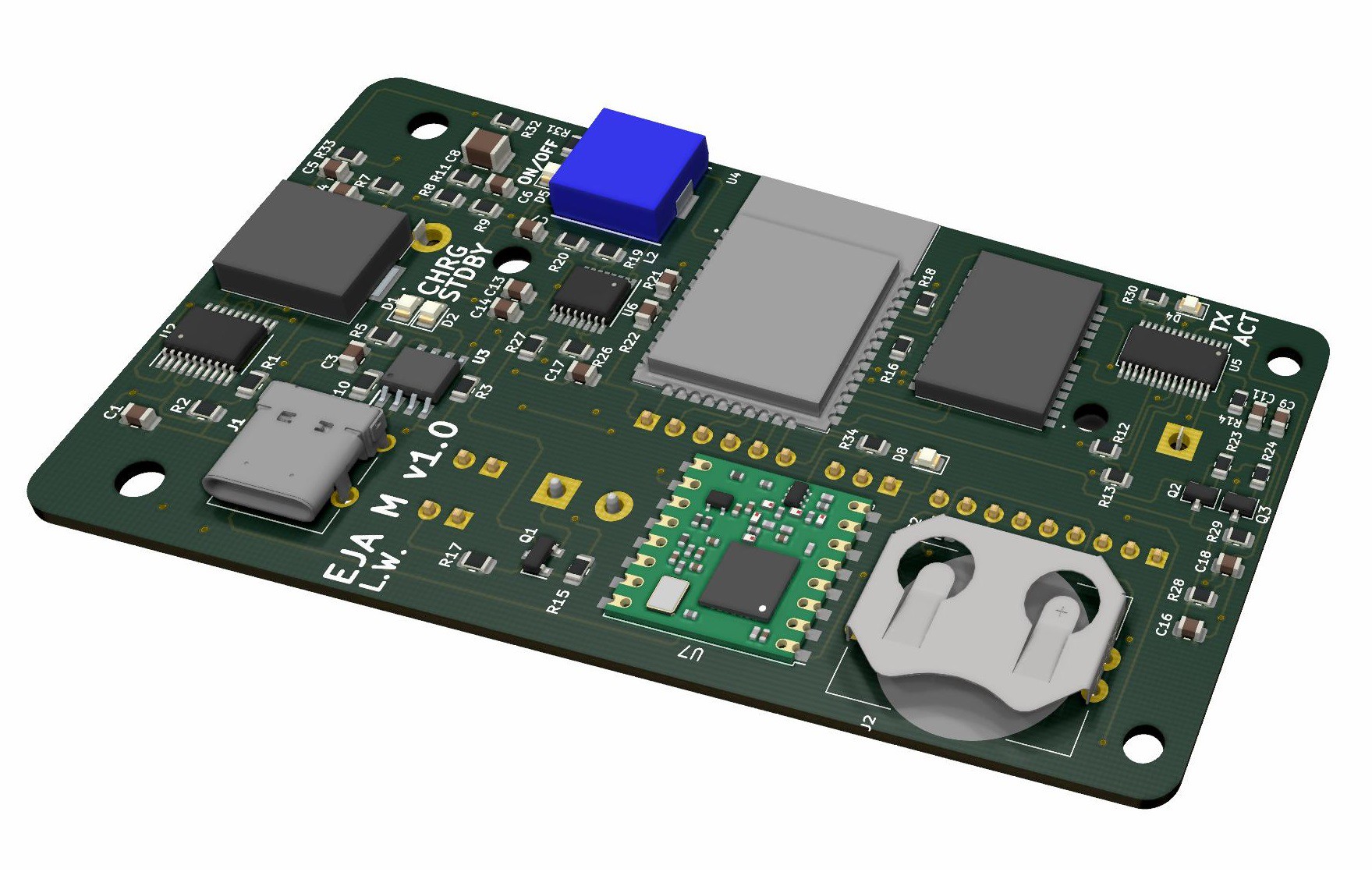
09/15/2021 at 16:43 • 0 comments![]()
We have a brand new PCB design, the EJA M v1.0 will replace our previous designs, it can be used as the Buoy or as the Onboard Gateway. The design includes the following features:
- USB C Port with Electromagnetic Compatibility (EMC)
- FTDI (FT260S-U) with an Auto Reset Circuit for the ESP32
- ESP32
- GPS Module
- LoRa Transceiver
- Real-time Clock (RTC)
- Connector for a Servo Motor
- 5V 2A Stepup (for the Servo Motor)
- 3.3V Battery Charging Circuit
- Connector for a 3 axis accelerometer
- Circuit to measure the battery level
- 3.3V 3A SEPIC Converter
- On-OFF circuit for a Button
- Access to unused pins in the ESP32
The design can be found in the following Github repository.
This log contains a more detailed description about the implementation of the different features in the design.
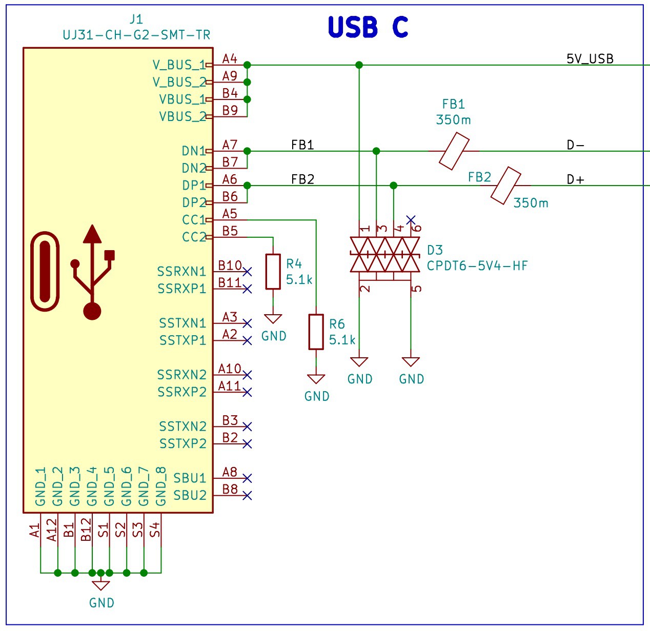
USB C Port with Electromagnetic Compatibility (EMC)
Everything starts with the USB C port, we have chosen this type of USB because it's size and because of the growing trend of using this port to charge and communicate with portable devices.
We have included Transient Voltage Suppression (TVS) diodes and Ferrite Beads to reduce the Electromagnetic Interference (EMI). These protections for the USB port will add compliance with the EMC regulations and standards from the Federal Communications Commission (FCC) and the European Union.
![]()
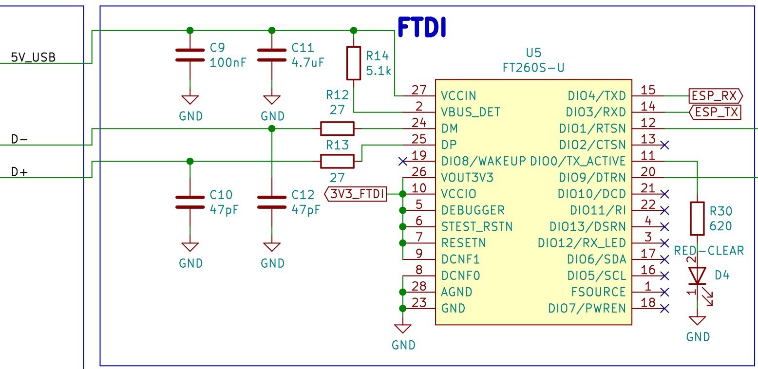
FTDI (FT260S-U)
The design includes the FT260S-U, a USB TO UART/I2C FTDI that will be used to program the ESP32.
![]()
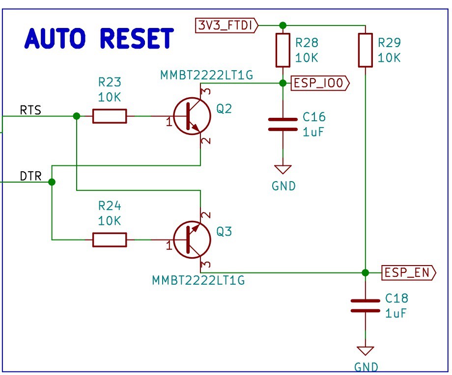
Auto Reset Circuit for the ESP32
The design includes an auto reset circuit that uses RTS and DTR to reset and put in bootloader mode the ESP32. For more information about this circuit, these blogs [1] [2] can be useful.
![]()
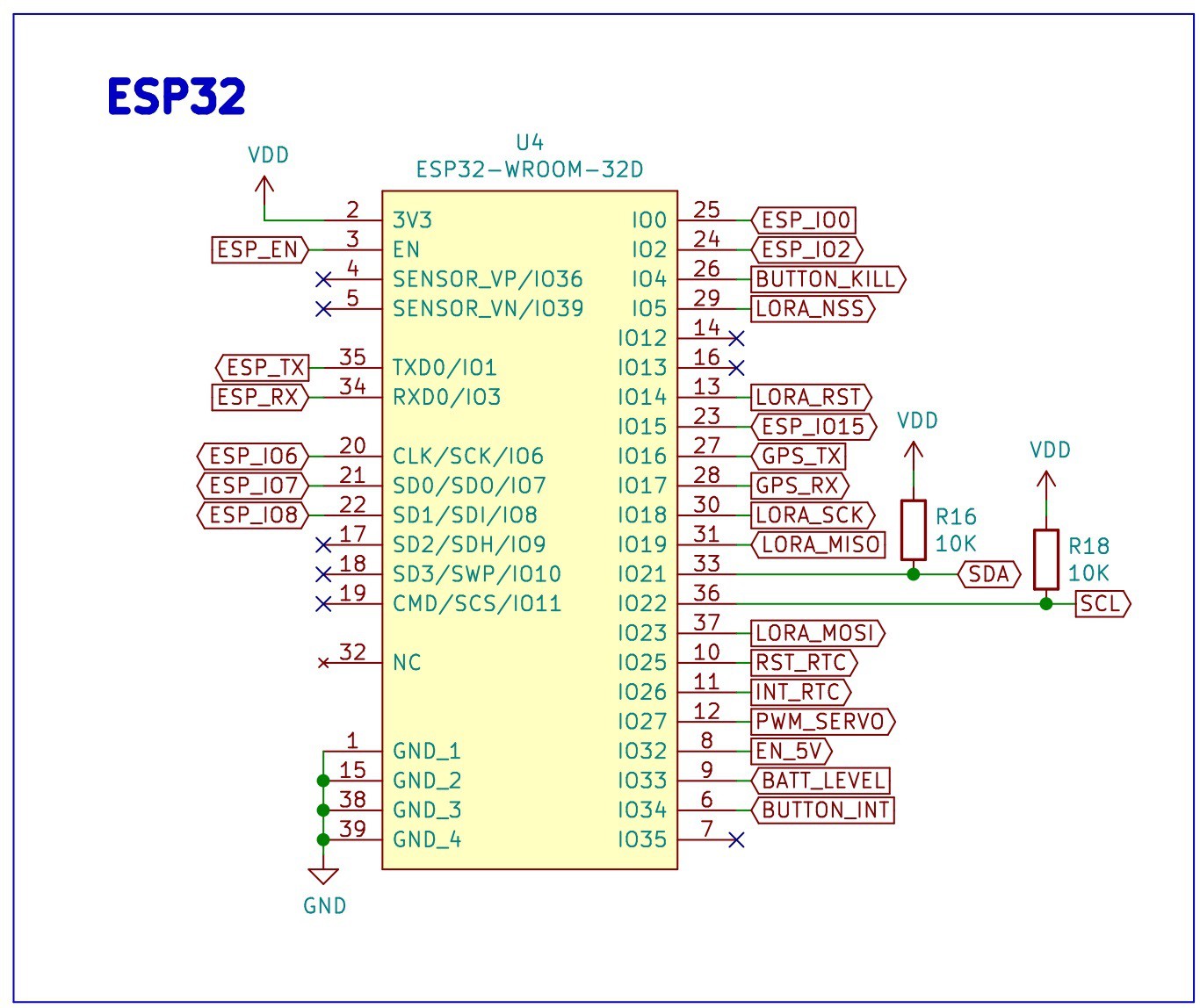
ESP32
The main microcontroller in the PCB is the ESP32, the following image shows the signals dedicated to the different pins. The ESP32 is connected to the FTDI, a GPS, a LoRa transceiver, a connector for a servo motor, a real-time clock, a circuit to measure the battery level, a connector for an accelerometer, and a few headers to provide access for the unused peripherals.
![]()
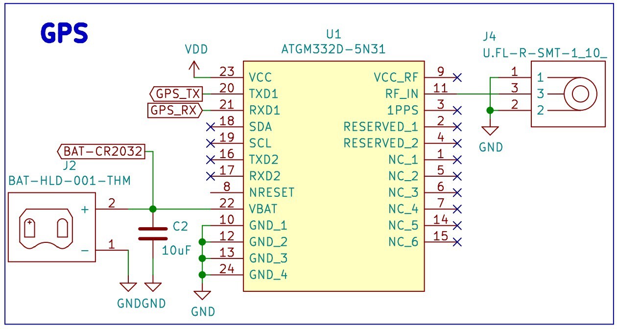
GPS
The selected GPS is the ATGM332D-5N31, one the modules tested previously in our Development Board for GPS Modules. The schematic is very simple, it has a decoupling capacitors (C2), a U.FL connector for an external antenna (J4) and a Coin Cell Battery Holder (J2).
![]()
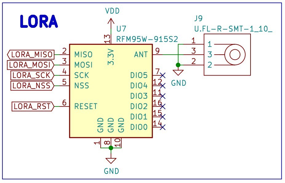
LoRa
The selected LoRa transceiver is the RFM95W-915S2, the same module tested in our Development Board for LoRa. The schematic contains a U.FL connector for an external antenna (J9).
![]()
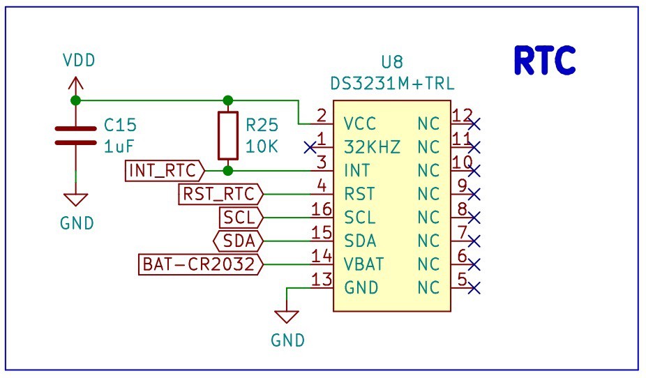
Real-time Clock (RTC)
The design includes a dedicated RTC, the DS3231M.
![]()
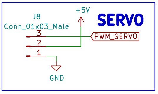
Servo Motor Connector
There is a 1x3 header connector for a Servo Motor, the 5V for the servo is provided by a 5V 2A Stepup.
![]()
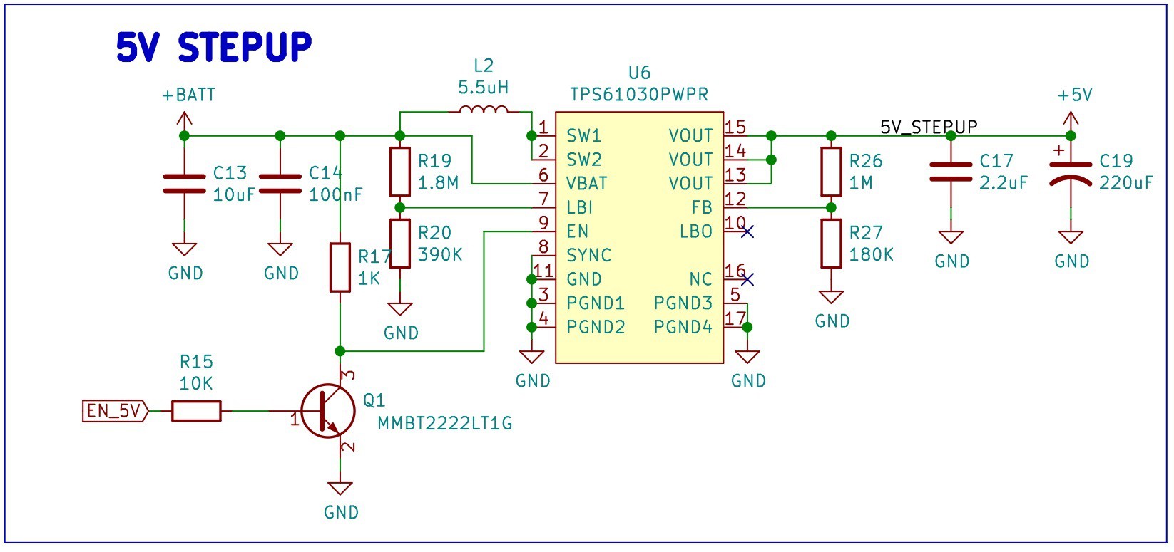
5V 2A Stepup
The design includes the TPS61030PWR, a boost converter with a 4A switch current, to provide the 5V for the Servo motor. The schematic contains the components for a 5V 2A output, following the design procedure that starts on the page 13 in the datasheet.
![]()
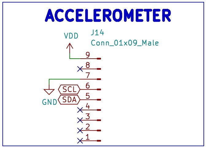
Accelerometer Connector
There is a connector for the ADXL343 3 axis accelerometer, a 1x9 header was used even though it only manages the signals VDD, GND, SCL and SDA, in case we want to use more connections for the accelerometer in future versions.
![]()
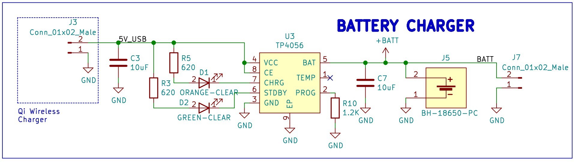
Battery Charging Circuit
To charge the 3.3V battery the design includes the TP4056, a 1A Standalone Linear Li-lon Battery Charger. The schematic includes a green led to show the user that the battery is charged and a red led to show the user that the battery is charging. There is a Battery Holder for a 18650 battery (J5) and an additional 1x2 header (J7) in case we want to use a different 3.3V battery. There is also a 1x2 header (J3) to use a different type of connection for the charger (instead of the USB C), for example we can connect and test a QI Wireless Charger.
![]()
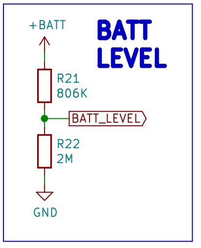
Battery Level
The design contains a circuit to measure a battery level, it is a simple resistor divider calculated for a range of 2.7V to 4.2V, the normal range for the 18650 Li-Ion Battery that will be used in the design.
![]()
Those values for the resistor divider give the following range for the ADC:
- Maximum voltage: 4.2V * (2M / (0.806M + 2M)) = 2.99V
- Minimum voltage: 2.7V * (2M / (0.806M + 2M)) = 1.92V
That means that the ADC from the ESP32 will be reading analog values from 1.92V to 2.99V from the battery measurement circuit.
For more information about measuring lithium battery voltage visit the following link.
3.3V 3A SEPIC Converter
Since the voltage of the battery can change from 2.7V (discharged) to 4.2V (charged), a SEPIC converter is included to provide a constant 3.3V to the digital circuits regardless of the changes in the input voltage from the battery. The selected SEPIC converter is the LTC3113EFE#TRPBF.
![]()
Note: The resistor R32 is a jumper that connects VDD to 3V3. R33 is a jumper that connects VDD to the battery. Do not solder both at the same time, it will create a short circuit between 3.3V from the SEPIC and the voltage from the battery. R32 and R33 are included just in case the SEPIC converter doesn't work and we have to connect the circuit directly to the battery.
Summary: Do not solder R33.
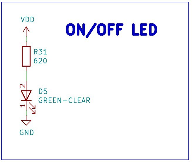
ON-OFF Led
There is Green Led that turns on with the 3.3V from the SEPIC converter, it will notify the user/developer that the device is ON or OFF.
![]()
ON/OFF Button Circuit
The design contains a LTC2954ITS8-1#TRPBF, a pushbutton ON/OFF controller that manages the power supply (enables the 3.3V SEPIC) via a pushbutton interface.
![]()
Extra Header
The design includes an 1x06 header to provide access for some of the unused pins in the ESP32.
![]()
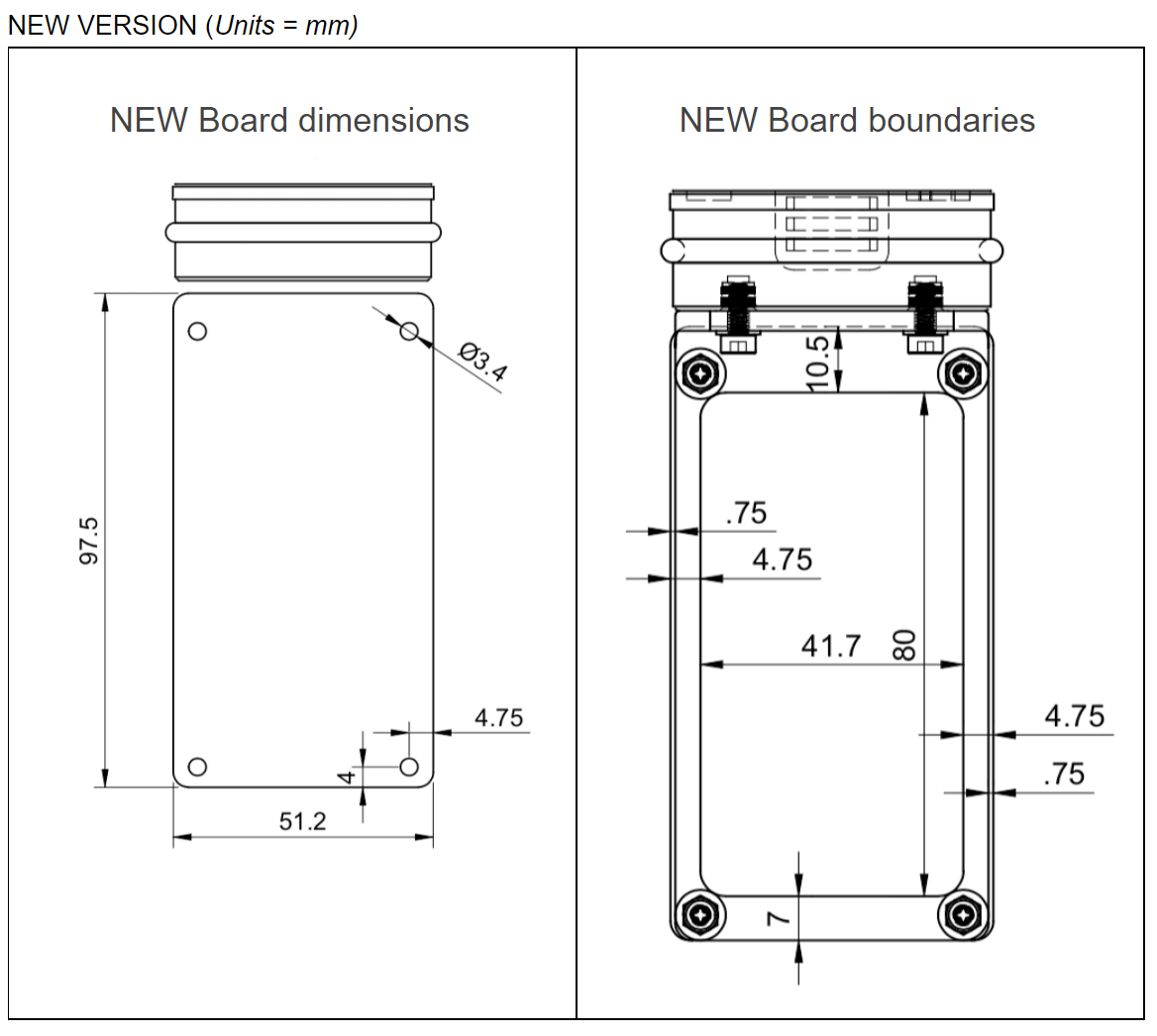
PCB Dimensions and Boundaries
The dimensions of the PCB are dictated by the maximum available space inside the buoy, from the enclosure design we where able to define the size of the PCB: 97.5 mm x 51.2 mm.
In the back layer there is a restricted region, that can't contain any components because the PCB is directly in contact with the enclosure in that region, those are the boundaries of the back layer. Through hole footprints where not be placed in that section, even if the footprint is placed in the front layer.
![]()
Final PCB
The following images show the front and back layers of the PCB.
![]()
![]()
2021 HDP Dream Team: EJA
Learn more about Team EJA's intelligent buoy, and how their solution will help the global fight against ghost gear.


 A: The beginning, getting oriented (see the buoy with different antenna orientations). Different ideas.
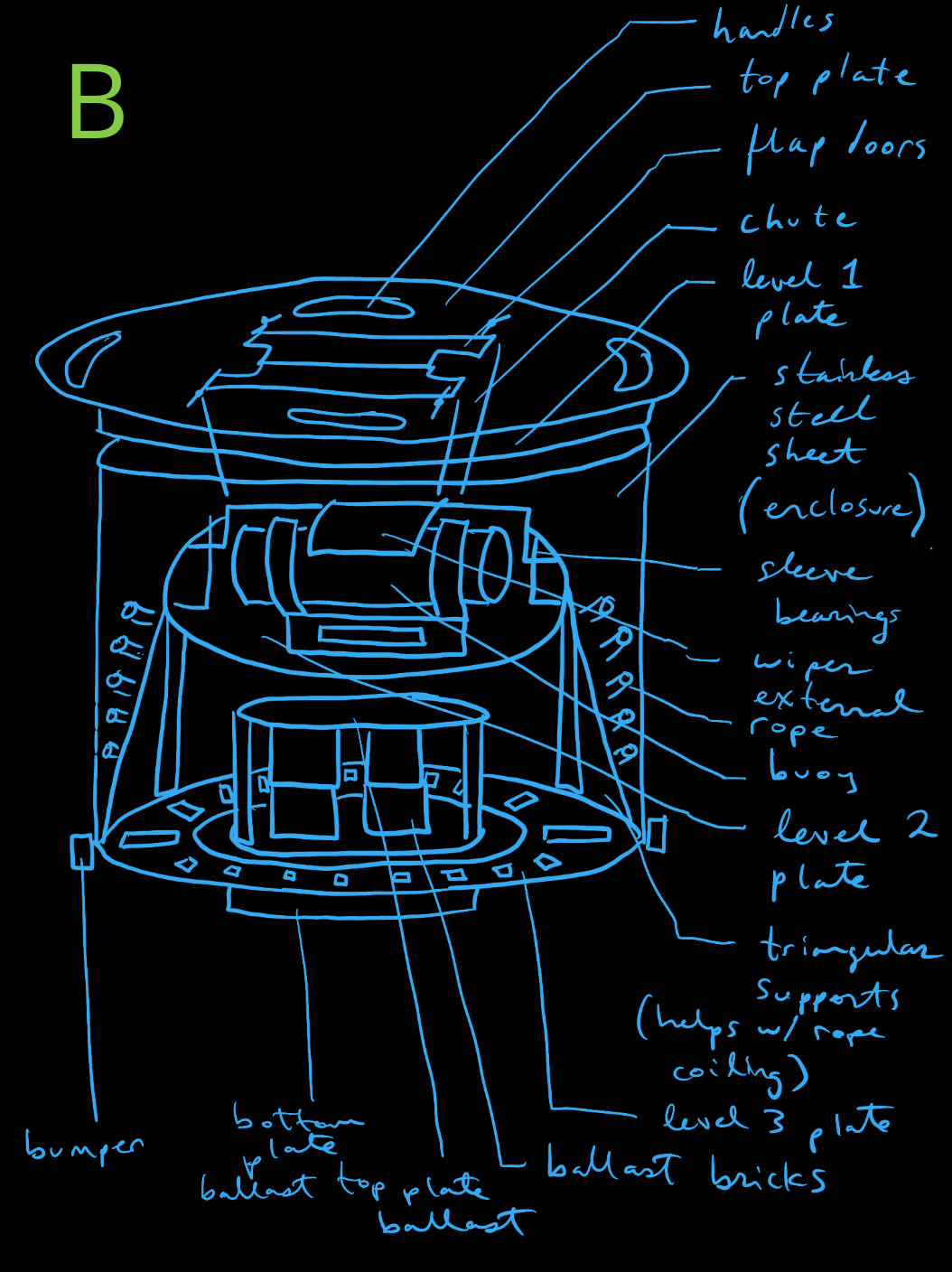 B: The somewhat finalized concept idea. This one had too many moving parts though. The commonality is the stacked stages.
 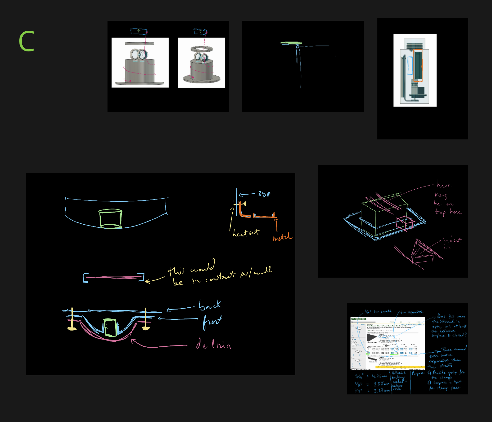 C: Wiper magnets being closer and with less friction with a thin delrin sheet. This idea was later scrapped since Giovanni came up with a great solution - two low-profile ‘rails’ that the wiper glides on - reducing scratches, minimizing contact area, and less materials!
 D: A lot of other ropeless fishing system designs use rope bags. What if there was a way to coil the rope? If it’s conical shaped, this would reduce tangling when coiling… however, if it is conical shaped, this means that the loading and landing orientation is 180 degrees flipped. This idea was scrapped because the centre of mass was at the top (for landing state, if it would even land like that).
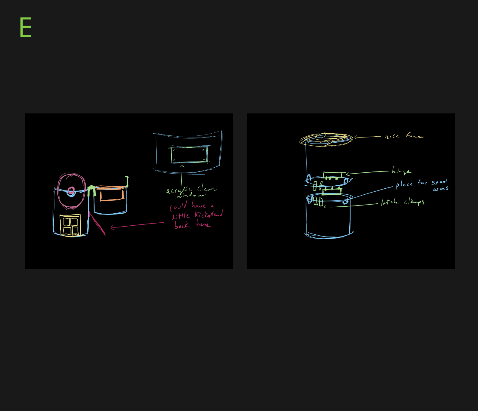 E: Here was another concept. It is a tube cut in half with latch clamps. This idea just didn’t work logistically, and it seems like it would be cumbersome to try to reload the spool afterwards.


 J: Electronics integration review with Leo! This was a great way to point out areas of concern on the integration side.