Fortunately the dynamics of the table are not too complicated. Let the state, x, of the table include 2 variables, position and velocity, x and v.
Given the relationship dx/dt = v, the state matrix equation is:
The only way to control the position is by changing the tilt of the table. We need to find the value of C such that it incorporates the relationship between the control input, u, the degree of tilt in the table, and the resulting acceleration on the ball. This relationship, including the small angle approximation of tilt angle (a = sin(theta) ≈ theta) and conversion to digitizer units, is all incorporated into the constant C.
In order to find C, the platform was tilted one unit to the right and the ball was rolled several times toward the left.
The timestamps and ball coordinates were sent to the serial port:
### Serial capture
### time (ms), x and y position (digitizer units)
102, 183, -60
201, 150, -63
302, 120, -65
402, 95, -65
502, 74, -65
602, 58, -66
702, 45, -66
802, 35, -65
902, 31, -66
1002, 30, -68
.... lots more lines
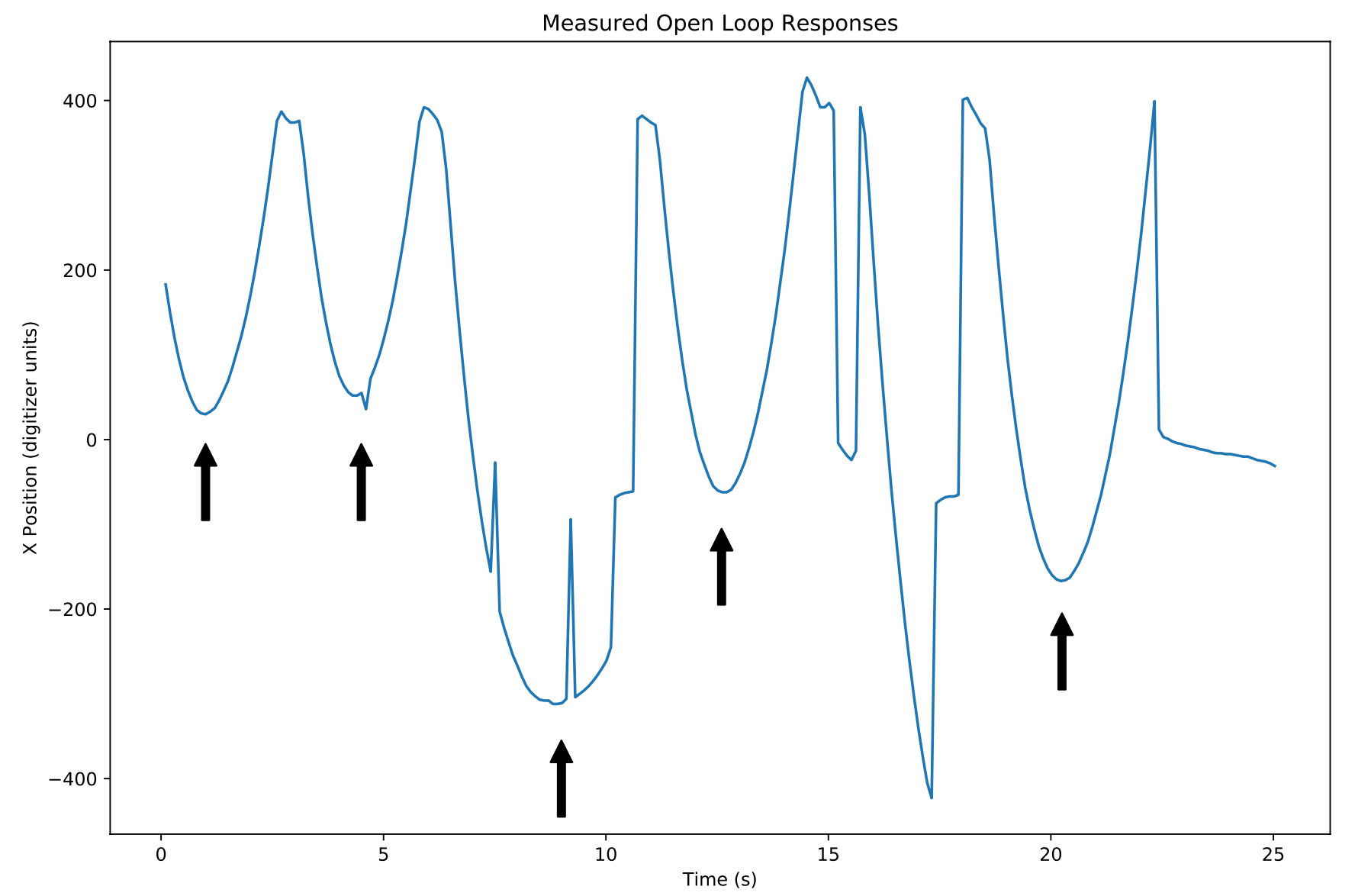
Which when plotted look like this:
Each of the black arrows point toward a ballistic trajectory, accelerating toward the positive x direction. You can see the occasional glitch in the position reading, likely due to dead spots in the transparent TIO (tin indium oxide) layer(s). One of these trajectories was chosen to fit the parameter C.
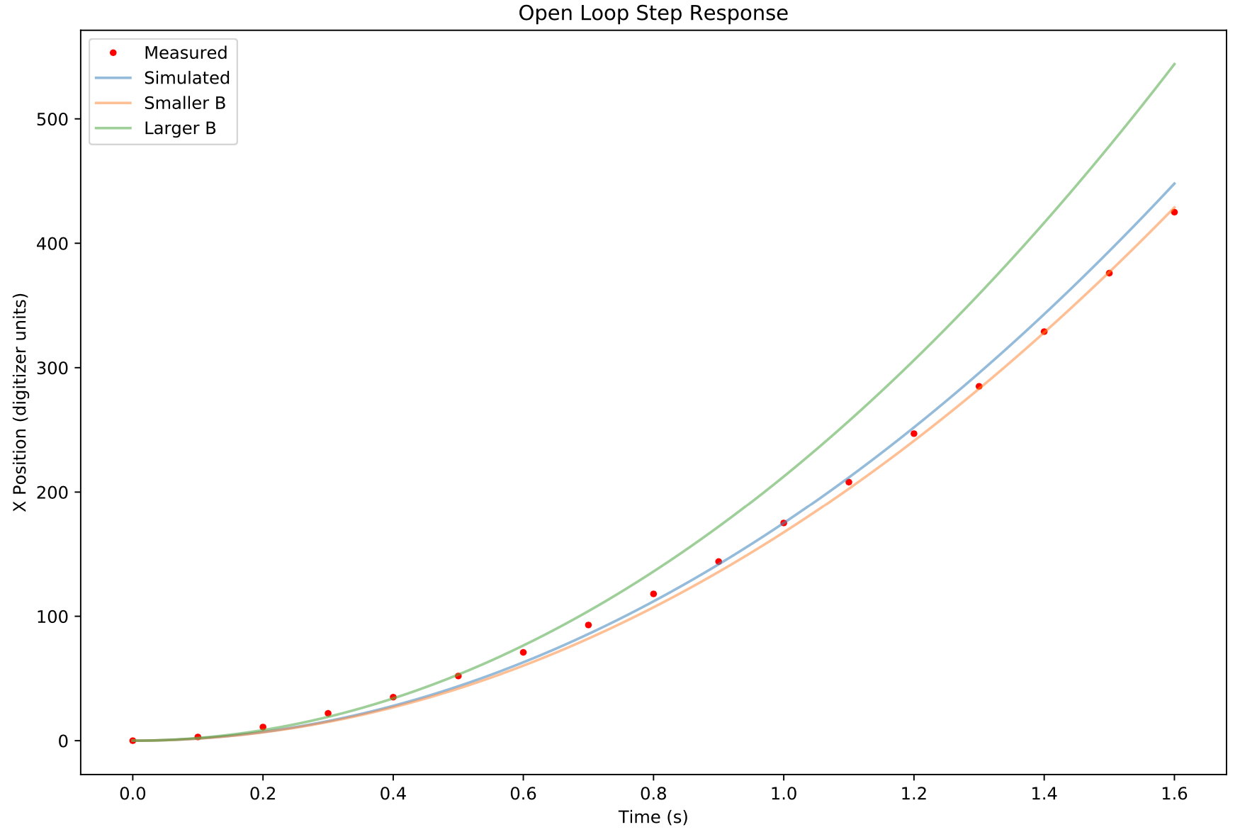
The red dots show the measured ball positions on the tilted table. The continuous lines show simulated step responses for various values of C.
The open loop system step response was simulated using the python control library control.step_response() function. As expected, when the table is tilted rightward, the ball accelerates to the right with a constant acceleration. And keeps going until it falls off the table.
It was not possible to get a perfect fit with the simplified model. The values shown above are for C= 335, 350, and 425 for the orange, blue, and green respectively. The blue, C=350, was chosen as a compromise. Perhaps the green would have been a better choice because it gives better short term approximations?
Convert to discrete time matrices using c2d( ) so that new states can be computed using
The Arduino is capable of ball measurements, the feedback calculations, and updating commands to the servos in about 5 ms which would allow a maximum update frequency of 200 Hz. Given that servos update at ~50Hz, it probably doesn't make sense to go all the way to 200 Hz.
I chose a relatively low Tstep value of 0.1 s, or 10 Hz update frequency with the idea that if you can't do it right slowly, doing it faster won't help. Get it working first, speed things up later.
I've glossed over some of the implementation details in the pursuit of space, but I have included all the ipython notebook files (and ball rolling data) so you can see and try this yourself. You may need to install a few libraries including numpy, matplotlib, and the python control library (https://python-control.readthedocs.io/en/0.8.3/).
Next up, feedback.
2
2. Adding Feedback
The videos on youtube discussing state space control make it seems simple: choose where you want your poles and as long as your system is controllable, you can find a feedback matrix that will get you where you want to go. In practice, there are plenty of details that can trip you up.
My path through state space was pieced together with studying and trial and error. Lather, rinse, repeat. If there are any real control engineers, I would welcome your feedback.
Using the place() command. The poles were placed on the left hand plane for stability but not too negative given the relatively slow update frequency.
poles = [-2.2, -2.]
Kfeedback = control.place(syst.A, syst.B, poles)
## which returns the following:[[0.01257143 0.012 ]]
The feedback matrix is 1x2 which when multiplied by the 2x1 full state variable, x, results in a scalar control input.
The new A matrix then becomes A - B * K
feedbackA = syst.A - syst.B@Kfeedback ## feedback system A matrix
sysFeedback = control.ss(feedbackA, syst.B, syst.C, 0)

T ,yout = control.step_response( sysFeedback)
The step response of the closed loop system no longer accelerates off the table.
For the three step responses above, the poles were placed at (-5 and -6), (-2.2 and -2), and (-1 and -0.8) for the orange, blue and green curves respectively. The faster responses require more control inputs and may not be stable with a low refresh rate. So the medium speed poles were chosen for now.
In addition to using the control library to simulate the response, I wanted to confirm that I could simulate and later control the system. This turned out to be simpler than I expected. The code basically looks like this:
x= np.matrix([[500], [0]])  ## initial value. 512 is max value of touchscreen.

yout = []
controls = []

for i in range(50):       ## simulate 5 seconds
    u =  -Kfeedback @ x
    x = sysd.A* x + sysd.B @ u  ## update system

    yout.append(x[0,0])        ## append position
    controls.append(u[0,0])    ## append control, u
Which basically boils down to two steps:
Calculate state feedback: u = -K * x
And update system: x = A * x + B * u
In this simulation, the full state is available. In the ball platform, the position is measured from the resistive touchscreen and the velocity can be computed as the Δ x divided by Tstep. The proper way, however, is to use something called an observer.
Full disclosure: The actual order of events was that I tried to implement a Kalman observer/filter. It was trickier than I thought. So I fell back to a "Luenberger" observer. I still plan on going back to a real Kalman observer to correct for the glitches in the touchscreen input.
It turns out that the observer is itself a state space system! Who knew!? In this system, the state variable is xhat or the estimated state.
xhat[k] = A * xhat[k-1] + B * U
N.B. the A and B for the observer are derived from the system matrices but not the same! Same for the observer U which is now 2x1 in size, the command input and the measured position.
The observer is found by calculating an observer gain for given set of desired poles:
poles = [-7, -8]
Kobs = control.place(syst.A.T, syst.C.T, poles).T
The .T notation performs a matrix transpose. The poles were chosen to be faster than the desired control response-- we want to be able to observe faster than we control. The returned Kobs gain is 2x1. It will be used to calculate the observer state matrices:
Aobs = A - K * C
Bobs is concatenation of B and K, i.e. the 2x1 matrices side by side.
The estimated state, xhat, will be:
xhat[k] = A * xhat[k-1] + B * u
N.B. These observer A and B matrices are different from the system matrices. Furthermore, the input, u, for the observer system has been augmented with a measured x, i.e. it is now a 2x1 matrix containing the input u from the ball/platform system, as well as the measured ball position.
This now allows us to do full state feedback using an incomplete state measurement-- in this example, only a position. The steps are:
Measure ball position
Construct observer u, namely system u from last iteration, and measured ball position
Feed this into the observer system to get new xhat which gives both position and velocity
Use xhat to compute full state feedback u
Control "real" system with this u
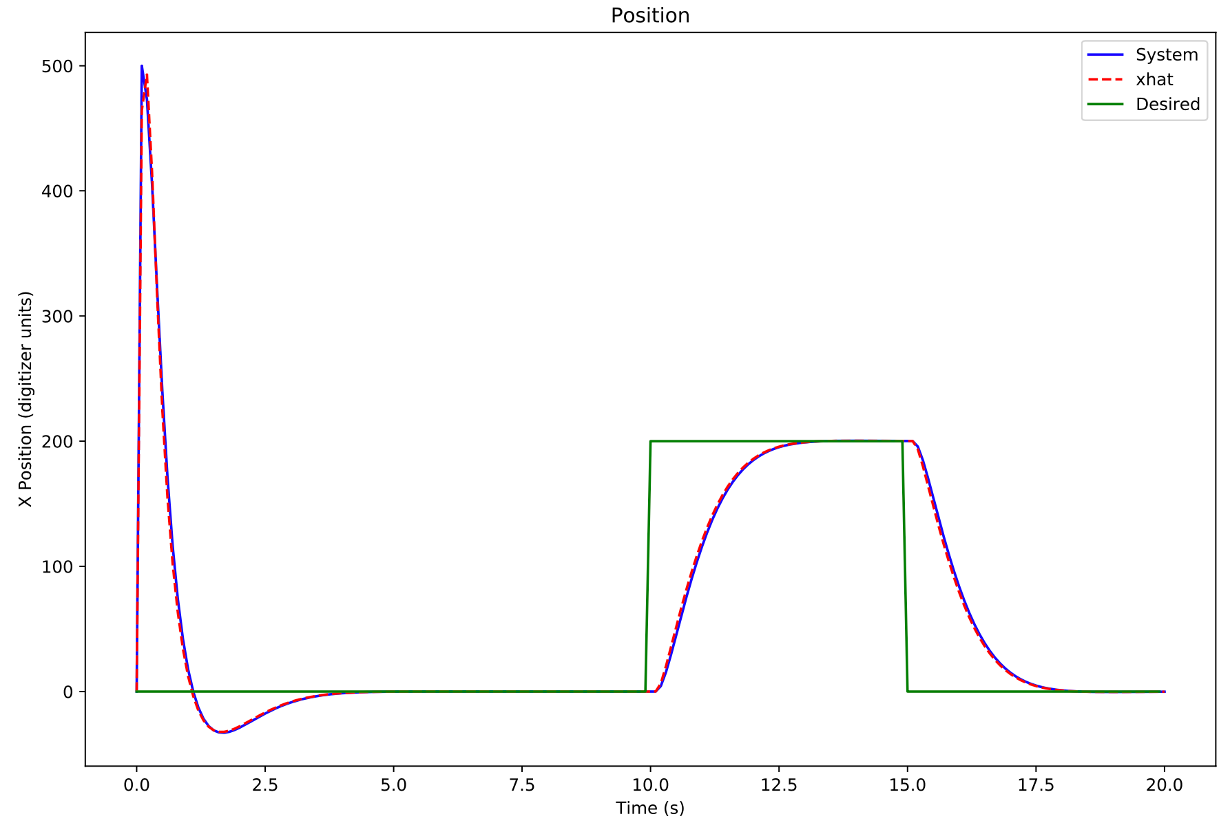
The plot above shows a manual simulation using an observer in the feedback loop. The green line is the command or desired position, the dashed red line is the xhat approximation, and the blue is the position of the "real system."
So the above code was converted into something the Arduino could handle and after a bit of fiddling, it would balance the ball. But the results were not what I expected, especially in regards to steady state error. The ball would stay on the table but thats about it. Deviation from ideal behavior, e.g. rolling friction, small offsets in table tilt, and imperfect model parameters made for lack-luster steady state response.
I had naively thought that state space control would automatically fix all such problems. It was a sobering realization. But what state space taketh away, state space giveth...
You can see the platform in action here:
BTW, all the python/jupyter notebooks used have been uploaded as well as the Arduino code.
Next up, robustness methods, namely, the addition of an integrator.
3
3. Robustness
So vanilla state feedback has problems with steady state error. It seems that one way of improving this is to use an integrator.
In broad brushstrokes, the plan is to compute an error signal and pass this through an integrator. This becomes an additional state, an accumulated error measurement. So now the state variable, x, goes from 2x1 to 3x1. There is a corresponding increase in size of the other state space matrices. You then choose feedback for this augmented state to make the integral of the error signal fall to zero. Boom. Easy.
In practice, how to do this was not no clear. It took a fair amount of searching and head scratching.
This part was not the easiest to understand, so please forgive any mistakes. I am sharing what I learned in the hopes that it may help others. If there are any control engineers reading this, I would welcome your feedback. In particular, when you calculate feedback, should the calculation be done using done continuous time matrices even though it is going to be used in discrete time?! No correction to improve on the discrepancy?
We will call this new integrated error signal sigma. Because x is now 3x1, all of the system matrices will need to be "augmented."
It took a while to understand how to implement this because if you try to construct a system with Aa, Ba, and Ca, it will return a system of order 2. At least that's what the python control library does. Likely because the system as defined is uncontrollable, i.e. third column of Aa and third row of Ba are all zero making the new sigma variable uncontrollable.
The solution? There are two augmented B matrices! Two of them! Ba is used to calculate the gain as well as compute the closed loop augmented A matrix. But in the closed loop system, the Br matrix is used. Who thinks up this stuff?!!
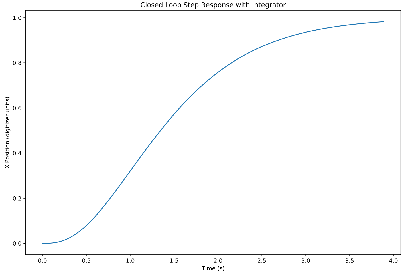
Once the integrator is incorporated into the control loop, the step response looks very similar to the response without the integrator:
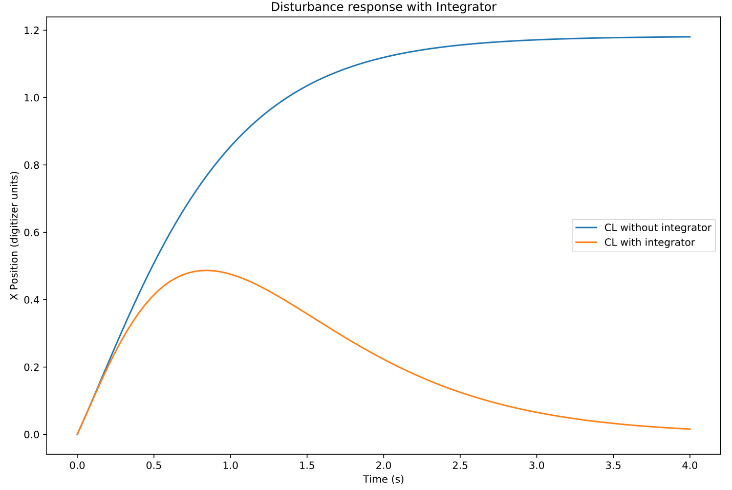
So what did we gain here? It looks indistinguishable from the original closed loop response? The difference comes in the disturbance response.
Where vanilla full state feedback (blue line) has significant steady state error, the incorporation of an integrator (orange) has much improved steady state error.
You can see the improves steady state response here (at 54 seconds):
I have uploaded the python notebook for anyone wanting to try this. The Arduino code is also available.
Up next, Kalman observer.
4
4. Kalman Observer
I previously mentioned glitches in position sensing, likely caused by "dead spots" in the TIO (tin indium oxide) layer(s) of the resistive touchscreen. The sudden apparent movement of the ball will cause the controller to react, sometimes causing the ball to fall off the platform. I will be exploring the use of a Kalman observer in the hopes of minimizing the effects of these glitches.
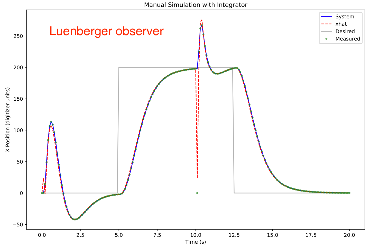
Shown below is the closed loop system response with a Luenberger observer. A sensor glitch to zero was simulated 10 s.
The grey line shows desired position, blue line shows the system position, red dotted line the xhat estimated position, and green the measured position which is the same as the system position except for at t =10 s.
The xhat estimated position is 90% toward the glitch value of zero. The control system corrects for the apparent position and velocity by tilting the table in the opposite direction. To address this issue a Kalman observer was implemented.
To construct the Kalman observer system, you will need to provide the system's A and C matrices just as for the Luenberger observer. But instead of placing the poles of this observer system, you need to provide (guesstimated?!) noise covariances. These will be used to calculate a feedback gain that is optimal in the sense of best linear estimation of the system given you have the correct system and noise characteristics.
You will need to provide a matrix for the state noise covariance, Vd, and another for the sensor noise covariance, Vn. If you make Vn (sensor noise covariance) high, the estimate will weight its state prediction more heavily and vice versa. I'll show the effects of changing these parameters later.
The observer K gain matrix is then computed using the control.lqe() function. It also returns the eigenvalues of the observer given those Vd and Vn parameters.
## This is the state noise covariance matrix
Vd = np.matrix([ [3, 0],
                [0, 3]])

Vn = 10 ## This is the sensor noise covariance

Kobs,P,E = control.lqe(A, Vd, C, Vd, Vn)
This will return a 2x1 matrix which is used the same as the Luenberger K matrix. Nothing else in the program needs to be changed to used this.
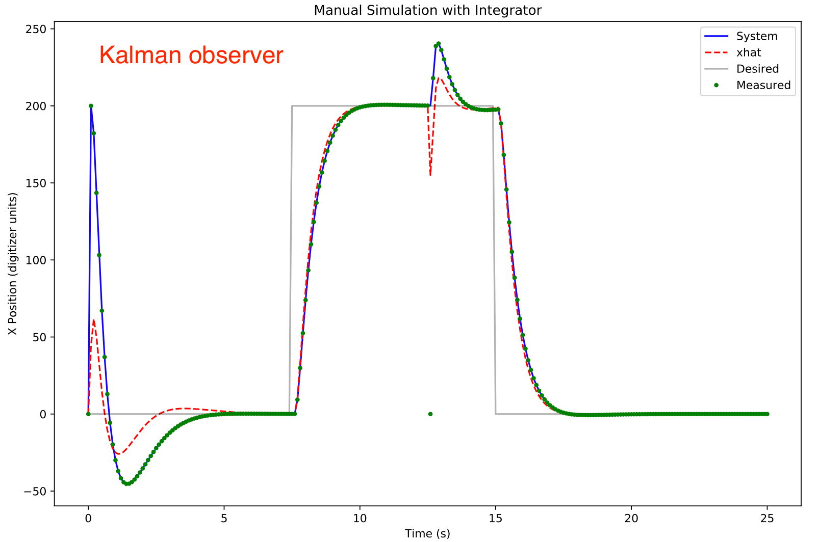
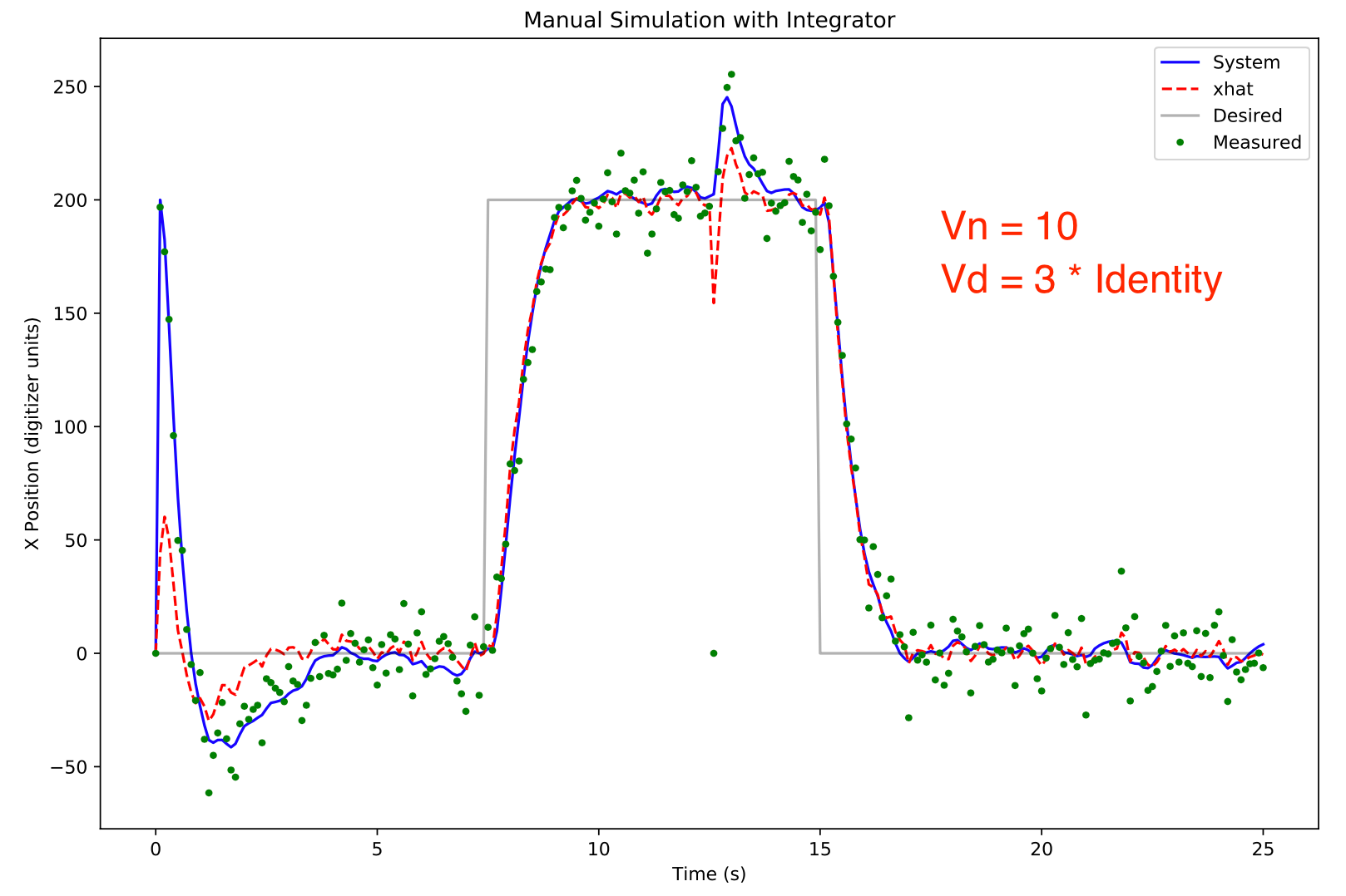
Shown below is the same feedback system using a Kalman observer with Vn = 10 and Vd = 3 * identity matrix:
With the Kalman observer, the glitch perturbation is markedly reduced. However, the observer takes considerably longer to start tracking the system, ~5 seconds.
To study the effects Vd and Vn on the Kalman observer, gaussian noise (variance 10) was added to the measurement. The xhat estimate was initialized to zero whereas the system position was 200. This allows observation of the system acquisition characteristics.
The xhat estimate from the Kalman observer is relatively immune to the effects of the noise.
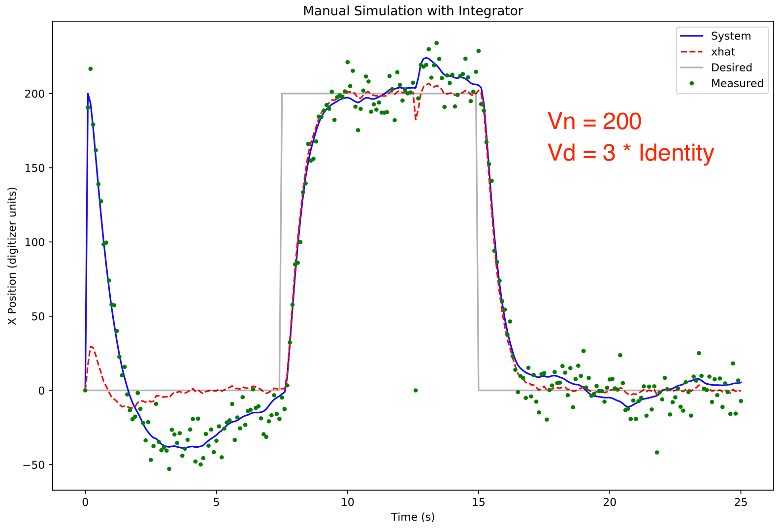
With Vn set to 200, the xhat estimate is even more noise and glitch resistant with the tradeoff being a very long acquisition time.
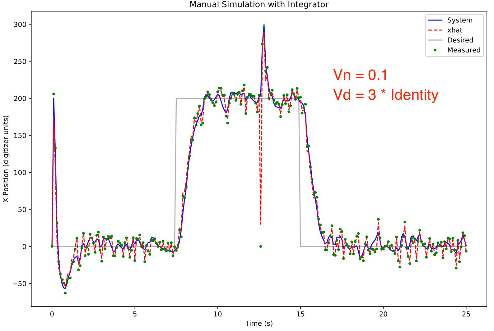
With Vn set to 0.1, the system acquisition time is almost immediate but almost all the noise and glitches are reflected in the xhat estimate. The Luenberger noise response looked very similar (data not shown).
So the ball balancing platform was changed to a Kalman observer with Vn = 10 and Vd = 3* identity matrix. Somewhat surprisingly the steady state error was once again huge despite using an integrator! What was happening was that the Kalman observer was returning a large value for the velocity even though the ball (and xhat position) was stationary. This was fixed by changing the Vd matrix to 3 and 20 along the diagonal. This forces the the Kalman observer to weigh its state velocity less heavily.
See the effects of the Kalman observer below (starting at 2:00):
 pjkim00

Discussions
Become a Hackaday.io Member
Create an account to leave a comment. Already have an account? Log In.