First, I have analyzed the computation of Graph SLAM step by step and then implemented the algorithm efficiently.

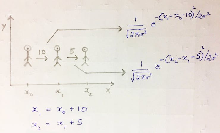
Assume a robot in the 2D world, tries to move 10 units to the right from x to x'. Due to motion uncertainty, x' = x + 10 may not hold, but it will be a Gaussian centered around x + 10. The Gaussian should peak when x’ approaches x + 10

If x1 is away from x0 by 10 units, the Kalman Filter models the uncertainty using the Gaussian with (x1 – x0 – 10). Hence, there is still a probability associated with locations < 10 and > 10.

There is another similar Gaussian at x2 with a higher spread. The total probability of the entire route is the product of the two Gaussians. We can drop the constants, as we just need to maximize the likelihood of the position x1, given x0. Thus the product of Gaussian becomes the sum of exponent terms, i.e. the constraint has only x’s and sigma.

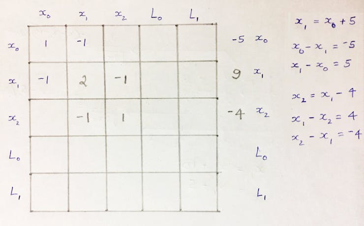
Graph SLAM models the constraints as System of Linear Equations (SLEs), with a Ω matrix containing the coefficients of the variables and a ξ vector that contains the limiting value of the constraints. Every time an observation is made between 2 poses, a 'local addition' is done on the 4 matrix elements (as the product of gaussian becomes the sum of exponents).

Let's say, the robot moves from x0 to x1 to x2 which are 5 and -4 units apart.

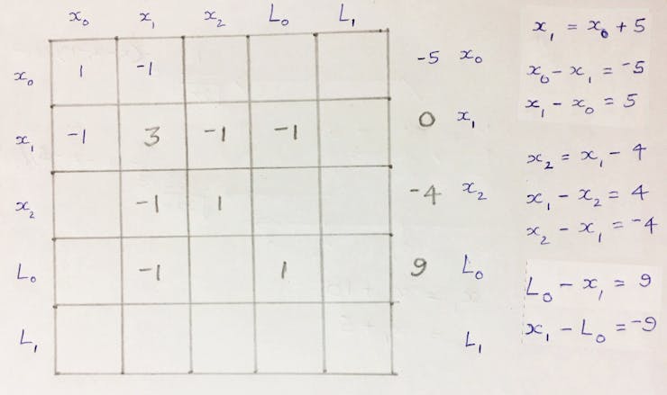
The coefficient of x’s and RHS values are added to corresponding cells. Consider the landmark L0 is at a distance of 9 units from x1.

Once the Ω matrix and ξ vector is filled in, as shown above, compute the equation below to get the best estimates of all the robot locations:

In order to do SLAM compute, you need to update the values in the 2D Ω matrix and ξ vector, to account for motion and measurement constraints in the x and y directions.

## Optimized implementation of Graph SLAM.

## slam takes in 6 arguments and returns mu, 
## mu is the entire path traversed by a robot (all x,y poses) *and* all landmarks locations
def slam(data, N, num_landmarks, world_size, motion_noise, measurement_noise):
    
    coefficients = [1, -1, -1, 1]
    
    # initialize the constraints
    initial_omega_1, initial_xi_1, initial_omega_2, initial_xi_2 = \\
                                   initialize_constraints(N, num_landmarks, world_size)
    
    ## get all the motion and measurement data as you iterate
    for i in range(len(data)):
        
        landmarks = data[i][0]  # measurement
        motion = data[i][1]  # motion
        
        # setting measurement constraints
        for landmark in landmarks:
            
            # calculate indices in the same order as coefficients (to meaningfully add)
            index1 = [i, i, N+landmark[0], N+landmark[0]]
            index2 = [i, N+landmark[0], i, N+landmark[0]]
            
            # dx update
            initial_omega_1[index1, index2] = initial_omega_1[index1, index2] + \\
                              np.divide(coefficients, measurement_noise)
            initial_xi_1[[i, N+landmark[0]]] = initial_xi_1[[i, N+landmark[0]]] + \\
                np.divide([-landmark[1], landmark[1]], measurement_noise)
            
            # dy update
            initial_omega_2[index1, index2] = initial_omega_2[index1, index2] + \\
                                        np.divide(coefficients, measurement_noise)
            initial_xi_2[[i, N+landmark[0]]] = initial_xi_2[[i, N+landmark[0]]] + \\
                          np.divide([-landmark[2], landmark[2]], measurement_noise)
        
        index1 = [i, i, i+1, i+1]
        index2 = [i, i+1, i, i+1]
        
        # dx update
        initial_omega_1[index1, index2] = initial_omega_1[index1, index2] + \\
                                       np.divide(coefficients, motion_noise)
        initial_xi_1[[i, i+1]] = initial_xi_1[[i, i+1]] + \\
                                np.divide([-motion[0], motion[0]], motion_noise)
        
        # dy update
        initial_omega_2[index1, index2] = initial_omega_2[index1, index2] + \\
                                       np.divide(coefficients, motion_noise)
        initial_xi_2[[i, i+1]] = initial_xi_2[[i, i+1]] + 
                            np.divide([-motion[1], motion[1]], motion_noise)
        
    ## To update the constraint matrix/vector to account for all measurements, 
    # measurement noise, motion and motion noise. Compute best estimate of poses
    # and landmark positions using the formula, omega_inverse * Xi
    mu_1 = np.linalg.inv(np.matrix(initial_omega_1)) * \\
                    np.expand_dims(initial_xi_1, 0).transpose()
    mu_2 = np.linalg.inv(np.matrix(initial_omega_2)) * \\
                    np.expand_dims(initial_xi_2, 0).transpose()
    
    mu = []
    for i in range(len(mu_1)):
        mu.extend((mu_1[i], mu_2[i]))
    
    return mu

 The complete source code and results of Custom SLAM implementation can be found in the IPython notebook here.

1) From the 2D LIDAR point cloud, use algorithms like Hough Transform to find the best fit line to generate floor maps.

2) From the 3D LIDAR point cloud, construct a 3D map of surroundings using Structure from Motion techniques,

• Use Detectors such as SIFT, SURF, ORB, Harris to find features like corners, gradients, edges, etc.
• Use Descriptors such as HOG to encode these features.
• Use Matchers such as FLANN to map features across images.
• Use 3D Triangulation to reconstruct a 3D Point Cloud.

3) We can use the idea of SLAM indoor navigation to deploy an autonomous mobile robot inside closed environments like airports, warehouses, or industrial plants.

4) SLAM navigation can be combined with Solution #5 (Navigation Assist for Blind & Elderly) and Solution #4 (Gesture Cam) to create a full-fledged Elderly Assistance Gadget that can not only help navigate but also understand the surrounding objects and even gestures made by the elderly. If deployed on an SoC with onboard IMU such as Pico4ML then the gadget can identify its own motion as a gesture.

Using PyRoboViz, I have visualized the 2D LIDAR map in real-time on Pi itself. However, while the visualization is on, the 'read descriptor bytes' from LIDAR occasionally flagged an error while scanning.

As a workaround, I have re-routed the real-time visualization of LIDAR map to a remote machine using MQTT. The robot position, angle, and map were encoded as a byte array that is decoded at the MQTT client as below.

# At the MQTT Transmission side

    data2Transmit = np.array([x, y, theta])

    # Map which is saved as a bytearray is appended at the end
    if scan_count % 30 == 0:
        client.publish("safetycam/topic/slamviz", \\
                           data2Transmit.tobytes() + mapbytes)
            
# At the MQTT receiving side

    # As 3 float values takes 8*3 = 24 bytes
    robotPos_bytes = msg.payload[:24]
    map_bytes = msg.payload[24:]

    robotPos = np.frombuffer(robotPos_bytes, dtype='float64')
    robotPos = np.array(robotPos)

    x, y, theta = robotPos
    viz.display(x / 1000., y / 1000., theta, map_bytes)

The only downside of this method is the slow rendering of the LIDAP map on the remote machine. You can increase the speed by reducing the MQTT publish frequency or reducing the map size. 

Later I found a better fix to the above 'read descriptor bytes' problem while scanning. The solution was to write the LIDAR scan method as a separate thread and keep the visualization as a separate thread while devising a mechanism for the threads to communicate.

The multi-threaded implementation can be found in the repository here

We can optimize power consumption based on the use case at hand. Even for the discussed solutions, alternate hardware can provide a more optimized implementation.

Let's discuss the power consumption of the above solutions under various settings.

a) Power Specification of Components

First, lets look at the power specification of each component used. Based on the measurements by RaspiTV and Pidramble [15] [16], here are some estimates:

• Raspberry Pi Zero (Idle) = 80mA * 5V = 0.4 W[Watts = Voltage x Current]
• Raspberry Pi 2B (Idle) = 220mA * 5V = 1.1 W
• Raspberry Pi 3B (Idle) = 260 mA * 5V = 1.4 W
• Raspberry Pi 4B (Idle) = 540 mA * 5V = 2.7 W
• RPi Zero 1.3 & Pi cam = 180 - 230 mA = 0.9 - 1.1 W (For 720p - 1080p)
• Raspberry Pi 3B and Pi cam = 460 mA * 5 = 2.3 W (To shoot 1080p video)
• Raspberry Pi 4B and Pi cam = 640 mA * 5 = 3.2 W (To shoot 1080p video)

You can drop the frame resolution of Pi Cam to save some power. RPi Cam draws 260 mA to shoot 1080p while only 180 mA for 720p. Raspberry Pi Zero 1.3 with Pi Cam draws only 0.9 W power while 720p video is being shot.

Now consider Movidius NCS and LIDAR,

• Movidius NCS 2 = 180 mA On 5V USB = 0.9 W

Based on RPLIDAR A1 Power Supply Specification [17],

• RPLIDAR A1 M8 = Scanner system + Motor system = 300 + 100 (Work Mode) * Voltage = 400 mA * 5V = 2W

For Door Access Control and Indoor Navigational Assistance use cases, you can usea Proximity Sensor instead of LIDAR.

• HC-SR04 Ultrasonic sensor = 15 mA * 5 = 75mW
• Grove Ultrasonic sensor = 8mA * 5 = 40 mW

For Luxonis OAK-D DepthAI Hardware, the total power consumption usually stays around 800-900ma, with cameras and the DepthAI SoM. The power expense of OpenMV Cam H7 is less than 150 ma andPico4ML is 40 ma in idle mode and 60 ma while running ML models.

b) Power Requirement of Solutions

The solutions with mathematical hacks are feasible to execute on Raspberry Pi Zero 1.3 at least power cost. It is trivial to port the above solutions across various models of Pi or OAK-D, as it supports OpenVINO and MYRIAD. Even to Depth AI hardware like OpenMV Cam H7 or Pico4ML, it is easy to port some use-cases with serious power gains.

The power requirement of ported, OAK-D, OpenMV Cam & Pico4ML are given under "Ported", "OAK-D", "Open MV", and "Pico4ML" heads respectively.

1) ADAS - Collision Avoidance System on Indian Cars

Better run this on a recent RPi model, as response time is critical here.

• Current: RPi 4B + Cam + Movidius + LIDAR = 3.2 + 0.9 + 2 = 6.1W
• Ported: RPi 3B + Cam + Movidius + LIDAR = 2.3 + 0.9 + 2 = 5.2 W
• OAK-D: RPi 3B + OAK-D = (260 + 800) * 5 = 5.3 W

2) Indoor Robot Localization with SLAM

If no point cloud visualization, it is enough to use Raspberry Pi 2B or 3B.

• Current: RPi 4B + LIDAR = 2.7 + 2 = 4.7W
• Ported: RPi 2B + LIDAR = 1.1 + 2 = 3.2W

3)Touch-less Attendance & Door Access Control

This solution can run on Raspberry Pi Zero 1.3with Movidius, though the frame rate can fall from 12-20 to 4-8 FPS which is decent enough. LIDAR can be replaced with an ultrasonic sensor for depth perception.

OpenMV Cam H7 has Haar Cascade Face Detection, but better to use DL for Face Recognition in a security use case. However, OpenMV Cam is a good alternative as eye-tracking & optical flow is handled in the hardware.

• Current: RPi 3B + Cam + NCS + LIDAR = 2.3 + 0.9 + 2 = 5.2W
• Ported: RPi 0 + Cam + NCS + U-sonic sensor = 80 + 180 + 180 + 8 =2.24 W
• OAK-D: RPi 3B + OAK-D = (260 + 800) * 5 = 5.3 W

4) Indoor Navigational Assistance for Blind & Elderly

This solution can easily be ported to Raspberry Pi 2B but it's ideal to use OAK-D here as it can do depth sensing, object detection, and tracking as well.

• Current: RPi 3B + Cam + Movidius = 2.3 + 0.9 = 3.2W
• OAK-D: RPi 2B + OAK-D = (220 + 800) * 5 = 5 W

5) Smart Cam with Gesture Alarm for Women Security

Our efficient solution based on linear algebra can be executed on Raspberry Pi Zero. However, OpenMV Cam is ideal for this use case, as it can do circle detection, and blob centroid detection based on color, in the hardware. However, you can fetch a huge power gain, if you use Pico4ML itself as the gesture object, as it has an IMU onboard.

• Current: RPi 3B + Cam = 460 mA * 5V = 2.3 W
• Ported: Raspberry Pi Zero 1.3 + Cam = 0.9W
• OpenMV: Less than 150 mA * 5V = 0.75 W
• Pico4ML: 50 mA * 5V = 0.25 W

6) Security Barrier Cam using Shape Context

The mathematical hack based on Shape Context can be executed on Raspberry Pi Zero, by replacing Pearson's chi-squared test with cosine distance to compare log-bin histograms.

• Current: RPi 3B + Cam = 460 mA * 5V = 2.3 W
• Ported: Raspberry Pi Zero 1.3 + Cam = 0.9W
• OAK-D: RPi 2B + OAK-D = (220 + 800) * 5 = 5 W

7) Monocular Social Distance Tracker

The depth inference and distance compute runs on another remote machine.

• Current: RPi 3B + Cam = 460 mA * 5V = 2.3 W
• Ported: Raspberry Pi Zero 1.3 + Cam = 0.9W

8) Worksite Helmet Monitoring

More industrial situations can be handled by adding Depth AI to this solution.

• Current: RPi 3B + Cam + Movidius = 2.3 + 0.9 = 3.2W
• OAK-D: RPi 2B + OAK-D = (220 + 800) * 5 = 5 W

WiFi may be required for some of the solutions above. Note that the Pi further consumes 170 mA when the wifi is turned on. To compensate, you can drop the frame resolution from 1080p to 720p to save nearly 100 mA. So the power expense remains more or less the same.

The speaker is an optional component in most of the use cases, even otherwise you can use a low-power USB speaker or audio HAT like this for sound. The Blinkt and LED SHIM are also optional components. Hence, they are not accounted for in the power expense computations.

c) Uptime Estimation on Battery

Let's try to estimate the uptime of the above implementations on battery, based on the power estimate under "Current" and "Ported" (considered same, as we can use the same code in another Pi model).

Battery uptime depends on the current draw. For 1000 mA current draw, a 10 Ah battery can last 10 hours.

Uptime in Hours = Battery Capacity (mAh) ÷ Current (mA)

Thus, on a 10 Ah battery, the above implementations,

• ADAS - Collision Avoidance System: can run 10 hours
• Indoor Robot Localization with SLAM: can run 15 hours
• Touch-less Attendance & Door Access Control: can run 22 hours
• Indoor Navigational Assistance for Blind & Elderly: can run 15 hours
• Smart Cam with Gesture Alarm for Women Security: can run 55 hours
• Security Barrier Cam using Shape Context: can run 55 hours
• MonocularSocial Distance Tracker: can run 15 hours

For some use cases, the actual up-time can be slightly lesser, as RPi draws more power under work mode. The OAK-D solution variant can last longer in real, as it draws only around 700-800 ma in work mode and much lesser in idle mode. Moreover, neural inference runs on OAK-D, freeing the host device resources.

However, note that both Gesture Cam and Security Barrier solutions qualify for always-on use cases, as they draw the least power, despite doing on-device sensor data analytics. Moreover, Gesture Cam can run 66 hours on OpenMV Cam H7, and around 200 hours on Pico4ML.

However, Pico4ML requires itself to be used to signal gestures, which may not be practical. Hence, OpenMV is the most ideal choice for Gesture Cam because it can do circle detection, and color mask on the hardware itself.

A very useful industrial solution could be the detection of people not wearing helmets in worksites and giving warnings for their safety. To demonstrate, see the output of the YOLOX model trained with this dataset using roboflow.

YOLOX is a high-performance YOLO, particularly suited for edge as it supports ONNX, TensorRT, and OpenVINO. Hardware optimization of the trained model to OpenVINO model is discussed in Solution #5.

I have implemented the below algorithm to solve a Depth AI use case - Social Distance Monitoring - using monocular images. The output of the algorithm is shown at the bottom.

a) Feed the input image frames every couple of seconds

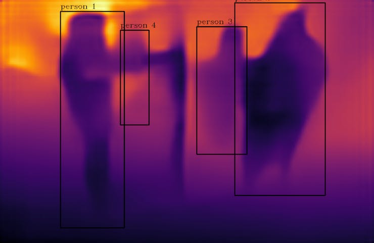
b) Fuse the disparity map with the object detection output, similar to visual sensor fusion. More concretely, find the depth of those pixels inside each object bounding box to compute the median to estimate the object depth.

c) Find the centroid of each object bounding box and map the corresponding depth to the object.

d) Across each object in the image, find the depth difference and also (x, y) axis difference. Multiply depth difference with a scaling factor.

e)Use the Pythagoras theorem to compute the Euclidean distance between each bounding box considering depth difference as one axis. The scaling factor for depth needs to be estimated during the initial camera calibration.

  # Detections contains bounding boxes using object detection model
  boxcount = 0
  depths = []
  bboxMidXs = []
  bboxMidYs = []
  # This is computed to reflect real distance during initial camera calibration
  scalingFactor = 1000 
  # Depth scaling factor is based on one-time cam calibration 
  for detection in detections:

      xmin, ymin, xmax, ymax = detection

      depths.append(np.median(disp[ymin:ymax, xmin:xmax]))
      bboxMidXs.append((xmin+xmax)/2)
      bboxMidYs.append((ymin+ymax)/2)

      size = disp.shape[:2]
      # disp = draw_detections(disp, detection)
      xmin = max(int(detection[0]), 0)
      ymin = max(int(detection[1]), 0)
      xmax = min(int(detection[2]), size[1])
      ymax = min(int(detection[3]), size[0])

      boxcount = boxcount + 1

      cv2.rectangle(disp, (xmin, ymin), (xmax, ymax), (0,255,0), 2)
      cv2.putText(disp, '{} {}'.format('person', boxcount),
               (xmin, ymin - 7), cv2.FONT_HERSHEY_COMPLEX, 0.6, (0,255,0), 1)


  for i in range(len(bboxMidXs)):
      for j in range(i+1, len(bboxMidXs)):
          dist = np.square(bboxMidXs[i] - bboxMidXs[j]) + 
                           np.square((depths[i]-depths[j])*scalingFactor)

          # check whether less than 200 to detect
          # social distance violations
          if np.sqrt(dist) < 200:
              color = (0, 0, 255)
              thickness = 3
          else:
              color = (0, 255, 0)
              thickness = 1

          cv2.line(original_img, (int(bboxMidXs[i]), int(bboxMidYs[i])), 
                (int(bboxMidXs[j]), int(bboxMidYs[j])), color, thickness)

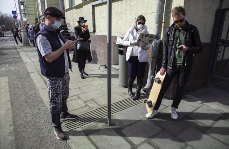
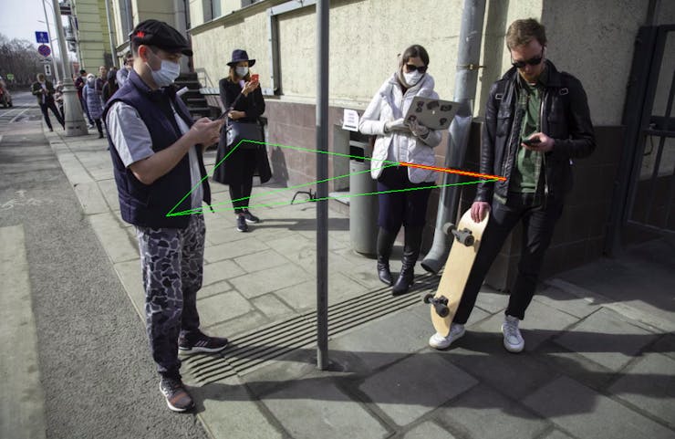
Input Image:

Disparity Map - Object Detection Fusion:

Output Image:

The people who don't adhere to minimum threshold distance are identified to be violating the social distancing norm, using a monocular camera image.

I have used computer vision to detect the license plate of the approaching car. Since the car comes near the security barrier to a predefined distance, we can predefine a minimum and maximum contour area to locate the license plate in an image.

img = cv2.imread("car.png")
gray = cv2.cvtColor(img, cv2.COLOR_BGR2GRAY)
ret, gray = cv2.threshold(gray, 250,255,0)

# applying different thresholding techniques on the input image
# all pixels value above 120 will be set to 255
ret, thresh2 = cv2.threshold(img, 120, 255, cv2.THRESH_BINARY_INV)
gray = cv2.cvtColor(thresh2, cv2.COLOR_BGR2GRAY)
contours, _ = cv2.findContours(gray, cv2.RETR_TREE, cv2.CHAIN_APPROX_SIMPLE)

for cnt in contours:
    approx = cv2.approxPolyDP(cnt, 0.01*cv2.arcLength(cnt, True), True)

    # The area constant is computed by the expectation of
    # how near the car can come near the security barrier
    if len(approx) == 4 and cv2.contourArea(cnt) > 1000:
        # Draw the License Plate Contour
        cv2.drawContours(img, [approx], 0, (0), 5) 

cv2.imshow("shapes", img)
cv2.waitKey(0)
cv2.destroyAllWindows()

We can use a combination of Deep Learning and Shape Context to detect and identify license plates. DL to detect the vehicle and corners of the license plate and Shape Context to recognize the alpha numerals in the license plate. See the OpenVINO model is able to detect the vehicle and license plate as shown below.

• After finding the corners of the license plate, compute the perspective transform matrix and warp the license plate to get a frontal projection.
• Preprocess the frontal image to get ROI and run contour detection. Filter unnecessary contours based on the shape and size of the contour.
• Apply shape context matching on each contour to identify the alphabets and numerals in the license plate.

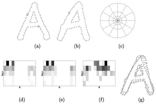
See the output of shape context detection on different Indian license plates:

The mathematical descriptor known as Shape Context uses log-polar histograms to encode relative shape information. This can be used to extract alphabet shapes from an image efficiently. The implemented algorithm is as below.

• Log-polar histogram bins are used to compute & compare shape contexts using Pearson’s chi-squared test [12]

• It captures the angle and distance to randomly sampled (n-1) points of a shape, from the reference point
• To identify an alphabet, find the pointwise correspondences between edges of an alphabet shape and stored base image alphabets. [12]

• To identify an alphabet or numeral, find character contours in an image. Filter out the contours based on size and shape to keep the relevant ones.
• Compare contours with each shape inside the base image. The base image contains all the potential characters, both alphabets, and numerals.
• Find the character with the lowest histogram match score
• Do the above for all character contours, to extract the whole text.

# This code builds the shape context descriptor, which is the core of our alphanumeral comparison
# https://github.com/AdroitAnandAI/Multilingual-Text-Inversion-Detection-of-Scanned-Images
        # points represents the edge shape
        t_points = len(points)
        # getting euclidian distance
        r_array = cdist(points, points)
        # for rotation invariant feature
        am = r_array.argmax()
        max_points = [am / t_points, am % t_points]
        # normalizing
        r_array_n = r_array / r_array.mean()
        # create log space
        r_bin_edges = np.logspace(np.log10(self.r_inner), np.log10(self.r_outer), self.nbins_r)
        r_array_q = np.zeros((t_points, t_points), dtype=int)

        for m in xrange(self.nbins_r):
            r_array_q += (r_array_n < r_bin_edges[m])

        fz = r_array_q > 0

        # getting angles in radians
        theta_array = cdist(points, points, lambda u, v: math.atan2((v[1] - u[1]), (v[0] - u[0])))
        norm_angle = theta_array[max_points[0], max_points[1]]

        # making angles matrix rotation invariant
        theta_array = (theta_array - norm_angle * (np.ones((t_points, t_points)) - np.identity(t_points)))
        # removing all very small values because of float operation
        theta_array[np.abs(theta_array) < 1e-7] = 0

        # 2Pi shifted because we need angels in [0,2Pi]
        theta_array_2 = theta_array + 2 * math.pi * (theta_array < 0)
        # Simple Quantization
        theta_array_q = (1 + np.floor(theta_array_2 / (2 * math.pi / self.nbins_theta))).astype(int)

        # building point descriptor based on angle and distance
        nbins = self.nbins_theta * self.nbins_r
        descriptor = np.zeros((t_points, nbins))
        for i in xrange(t_points):
            sn = np.zeros((self.nbins_r, self.nbins_theta))
            for j in xrange(t_points):
                if (fz[i, j]):
                    sn[r_array_q[i, j] - 1, theta_array_q[i, j] - 1] += 1
            descriptor[i] = sn.reshape(nbins)