 Adam Spontarelli
Despite all of your friends who like to say that "heat goes up", heat actual moves according to this equation,
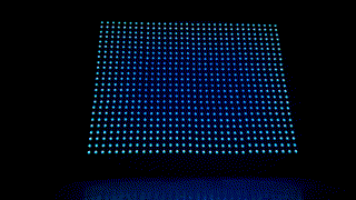
If you're wondering what on earth that means, you have two options: study differential equations for a few years or watch the colors change on our LED board. This LED board displays our solution to the 2D heat equation, written in less than 1Kb of program space. If you were to heat up a 14.5 x 10.9 inch sheet of copper, the heat would move through it exactly as our board displays. The same temperatures would be at the same locations at the same time. Don't believe it? Grab your thermocouple and come along!
The Setup
We built a 32x24 RGB LED matrix and attached six thermistors to the border. The temperature readings from the thermistors serve as the real-time boundary conditions to the solver, while the solution is displayed by the LEDs. In the video below we're heating the thermistors with a heatgun.
Solution
In order to solve this differential equation, you first need to approximate it as an algebraic equation. We chose to use a first order, forward difference in time and a second order central difference in space. The equation to solve then becomes,
Since the distance between the LEDs in the x-direction is the same as the y-direction on our display board, we can simplify a bit.
Much better. Now we use Euler's Explicit method to solve for the temperature.
And there you have it, the temperature at each node as a function of time. Assign boundary conditions, the appropriate distance between LEDs, use a thermal diffusivity associated with a material of your liking (we chose copper), and take a time step that doesn't violate the Courant Limit.
Code
We coded the solution in five main steps.
- Read the thermistors
- Update the boundary conditions
- Solve the conduction equation
- Update the LED color
- Wait for the appropriate amount of real time to pass before continuing
To see the code in all its glory head over to Github:
https://github.com/VectorSpaceHQ/2d_conduction
Code Size
The following output generated by running make in the avr/src
directory shows that when compiled with avr-gcc version 4.9.2 the
binary size of the program falls less than or equal to 1kB. 1024 bytes
exactly
avr-gcc --version
avr-gcc (GCC) 4.9.2
Copyright (C) 2014 Free Software Foundation, Inc.
This is free software; see the source for copying conditions.  There is NO
warranty; not even for MERCHANTABILITY or FITNESS FOR A PARTICULAR PURPOSE.

avr-gcc -mmcu=atmega328p -std=gnu99 -Os -ffunction-sections -fdata-sections -Wl,--gc-sections -Wl,-Map=conduction.map -flto -mrelax -lm -nostartfiles -g3 -DNO_VECTORS -DF_CPU=16000000 -I startup/common main.c spi.c adc.c rgb_matrix.c colormap.c conduction.c timer.c interpolate.c startup/crt1/gcrt1.S -o conduction
avr-size conduction
   text    data     bss     dec     hex filename
   1024        0    1600    2624     a40 conduction
avr-objcopy -O ihex -R .eeprom conduction conduction.hex
Size Reduction Techniques
We are using the AVR flavor of GCC as our compiler, and have made a few tweaks to help with the 1kB size constraint
- Used fixed point math instead of floating point
- Ask GCC to perform its usual optimizations for size
-Os - Create separate function and data sections in the executable and instruct the linker to garbage collect any unused sections:
-ffunction-sections -fdata-sections -Wl,--gc-sections - Allow for standard link-time optimization by asking GCC to save some of its internal representations to the object file of each compilation unit
-flto - Disable the standard system startup files when linking the final executable. We've created our own in src/startup and modified crt1/gcrt1.S to remove the code for the interrupt vectors since we won't be needing them for our project.
-nostartfiles

 davedarko
 Pierre-Loup M.
 ndGarage
 Michał Nowotka
This is a great interactive visualization! It's like some kind of thermal augmented reality. I could see this becoming a science museum exhibit.
I remember having to implement this algorithm in FORTRAN as an undergrad in 1988. We were the last engineering class they taught FORTRAN. They started using C after that.