A short video showing how I've managed to get consistent impacts by building a cardboard Da Vinci hammer can be found here:
Exploring the internals of trees with sound
Time-of-flight, tomography and more
Time-of-flight, tomography and more
To make the experience fit your profile, pick a username and tell us what interests you.
We found and based on your interests.
A short video showing how I've managed to get consistent impacts by building a cardboard Da Vinci hammer can be found here:
I've been using The 2x4 of Science as a test article for this project. Three piezo sensors were clamped in place on it:
(Ignore the holes for now. I'm not always great about taking pictures as I go.)
A is on the right; B is in the middle; C is on the left. The red lines are 5 cm apart. Here's a table showing the distances they're set at:
| Sensor C | 5 cm |
| Sensor B | 35 cm |
| Sensor A | 80 cm |
| Hammer impact | 100 cm |
Thus, the distances for the three segments are:
And since the hammer is at the 100cm mark, the vibration should hit A, then B, then C.
Data capture is, at the moment, tedious. I hook up the pico to my laptop, hook up two of the sensors (say, A and B) and start a screen session. I do a batch of 20 impacts; the timing for each one gets printed to my terminal: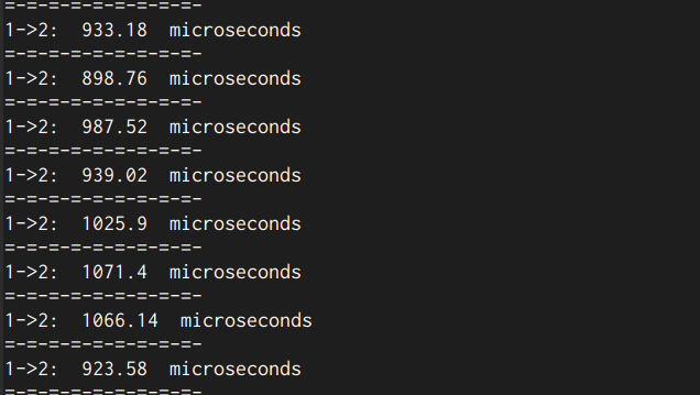
For extra fun, I made a point of tearing down the equipment between each run: disconnecting the sensors and the pico, taking the 2x4 of Science off the desk, then putting it all back together. I wanted to see if there was any difference being introduced by moving the equipment around.
And what did I find? Here's a strip graph (I think that's the right term) showing the results of 80 runs:
The Y axis is microseconds. For each segment the red dots are individual times, and the black dot is the mean. Remember, the hammer was beyond the A sensor, and vibration travelled from A → B → C. Here's what I notice:
| Sensor C | 5 cm |
| Sensor B | 35 cm |
| Hammer impact | 55 cm |
Also notice how the absolute time has changed: there's still about 200 microseconds between the groups, but now they're at ~525 and ~740 microseconds in this trial, vs 300 and 500 microseconds in the first.
I have a couple questions here:
After the initial exploration, I found some problems with the setup I used:
I decided to look for something new...and found it, thanks to a Pi Pico that my father had given me as a gift. I started looking for ways I could do high-resolution timing with it, and came across this thread in the Raspberry Pi forums that had pretty much exactly what I needed: example code that would do microsecond-resolution timing...and in microPython, no less! I had not done any reading on the capabilities of the Pico, and the state machine blew my mind. The example code posted by one of the folks in the thread was an excellent introduction to what could be accomplished; after a few hours of reading through the excellent SDK documentation, I thought I could get the timing I needed.
(Side note: the friendliness on display in the Pi forums, at least from what I saw, was amazing. It stands in unbelievably stark contrast to the unrelenting crankiness in seemingly every post I come across on the Arduino forums -- to the point where I now ignore search engine results that take me there, because the result will usually be unhelpful and depressing. Well done, Raspberry Pi folk.)
Meanwhile, I switched to using piezo sensors I had ordered from AliExpress:
I wanted to get something that was easy to hook up (love those pre-soldered header pins), and the adjustable threshold meant I could get it to act as a simple vibration detector, rather than measuring the vibration. One thing I didn't anticipate, though, is that the attachment of the piezo wires to the board is extremely fragile; the wires are quite thin, and are not well-secured to the board. I quickly broke 3 just by moving them around; a short attempt to resolder one didn't work (operator error, I'm sure). Fortunately I'd ordered 10, so I added electrical tape to them to give them a bit more structural integrity:
So! After some futzing around, I had:
With this setup, I started gathering data by knocking on the board and capturing the timing between different sensors as the sound travelled through:
(Side note: BEHOLD MY MIGHTY DIAGRAM.)
I was able to measure the time of flight successfully -- yay! -- but there was still a lot of variation when hammering by hand: for one set of measurements, it was anywhere between 855 and 1095 microseconds to travel 30cm. That's about a 25-30% difference. I tried dropping the hammer from the same height, but that really didn't do much.
I decided to assume for the moment that the code was okay, and try to eliminate the variation in the impact. I did more looking, and came across the Da Vinci hammer. There were lots of variations, but this video really inspired me:
Why do I say inspired? Because I'm a sysadmin by trade, and I'm not exaggerating when I say that I find it amazing that people can make matter do what they want. But this! It's hot glue and cardboard! I can do this! This video is glorious, and I really want to hold on to that sense of revelation. Here's the one I made:
Contents: some leftover cardboard packaging, a wooden spoon nationalized from the kitchen, a pen and a pencil to use for axes, and a steel rod bent into shape for a handle. I love it.
The result? The timing became immensely more consistent: I could get within 20 microseconds easily, and with some practice within 10 microseconds. There were slight variations in how the hammer/wooden...
Read more »First paper: Elastic wave modes for the assessment of structural timber: Ultrasonic echo for building elements and guided waves for pole and pile structures (DOI: https://doi.org/10.1007/s13349-014-0087-2, though that goes to a paywalled copy) by Martin Krause, Ulrike Dackermann and Jianchun Li. This had a lot of good background on sound propagation in wood and ultrasonic tomography. It also covered the topic of reflections of ultrasonic pulses -- which is something I'm starting to wonder about.
What's really good here, though, is the section on guided waves -- waves generated in a finite body (here, they consider pilings) that reflect both off the end of the body and off discontinuities or changes in structure:
Here, "SE" is sonic echo; "BW" is bending wave. "IR", a third method not in that diagram, is impulse response. Sonic echo and impulse response use the same testing method: hammering the end of the pile. The difference is in how the data is analyzed: time (SE) vs frequency (IR). By contrast, BW hammers the side of the pile, sending a bending wave down the structure; multiple sensors are used to measure the reflected waves.
The guided wave technique seems closest to what I have in mind -- at least for initial testing with the 2x4 of Science(tm) -- and this section is quite valuable. So is the table of velocities in different sorts of wood:
The consideration of choice of impact device (hammer to you and me) is also interesting:
For the SE method, an ordinary hammer is sufficient, while for the IR method and the BW method, a modally tuned impact hammer equipped with a load cell is beneficial to capture the force of the impact needed to calculate FRF data. An important feature of the hammer is the type of the hammer tip (hard, medium or soft). While hard tips produce high energy signals at high frequencies, soft tips generate lower energy signals at lower frequencies. In general, it is important to execute an impact that produces a frequency spectrum that provides adequate information for GW analysis. For SE/IR testing, it is recommended to generate an impact with a frequency range of up to 5000 Hz, while for BW testing, frequencies up to 3000 Hz should be excited. A higher excitation frequency bandwidth can also be achieved by mounting a steel plate or inserting a steel bolt to the timber pile/pole and inducing the hammer impact at the steel plate or steel bolt. To generate high quality wave data, the hammer impact should produce signals of minimal signal attenuation. The researchers Pandey & Anthony [40] found that a hammer of about 1.4 kg with a medium density plastic tip produces a good combination of signal energy with minimal signal attenuation for high quality signal data.
Overall, a very interesting paper that's only slightly intimidating. 😅
Next up, the closest paper to what I have in mind: In situ assessment of structural timber using stress-wave measurements (DOI: https://doi.org/10.1617/s11527-013-0095-4, though again that goes to a paywalled version) by Dackermann, U., Crews, K., Kasal, B. et al. Just look at figure 1:
This paper has some pretty practical considerations laid out: repetition of impacts to get average results (and throwing away the first measurement), considering moisture content and temperature, and my favourite part:
In general, if the stress wave velocity is lower than 10 % of the reference value or measurement results are fluctuating, the timber section should be suspected of having internal decay.
Off by an order of magnitude from what you were expecting? There might be some decay. 🤣 (The velocity table they include in this paper is the same as the one from the previous paper, BTW.) To be fair, they do outline all the things that go into that: transverse waves (left-hand illustration in figure 1) go about 1/5 to 1/3 the longitudinal speed; waiting for piezo sensors to warm up; and orientation...
Read more »In the course of researching this project, I came across a number of papers that covered the topic...or at least made interesting reading.
The first was Enhancing TreeMMoSys with a high-precision strain gauge to measure the wind-induced response of trees down to the ground, by Julius Nikl, Sven Kolbe and Dirk Schindler. This open access paper covered the use of strain gauges to measure wind load on trees. It wasn't exactly related to tree tomography, but it looks darn cool and it was the first time I'd come across strain gauges. Check out figure 6:
(This paper is from HardwareX, which is an open access scientific hardware journal; it is a vast, vast maze of rabbit holes and fun projects.)
Not exactly what I was looking for -- I don't have a tree in my yard, and I suspect that attaching aluminum bars to trees in my local parks would cause talk. But an interesting read nonetheless.
Next up was An automated sonic tomography system for the inspection of historical masonry walls by Ortega J, Meersman MFL, Aparicio S et al. This used a "scanning laser vibrometer" to pick up the vibrations from their "hitting device" (I love this simple term), which used a solenoid to arm, then release a spring-loaded head:
The hitting device moves around on a robotic frame to hit different parts of the masonry:
This allows it to tap the wall at precise grid points.
The paper goes into some detail on the signal processing, which I suspect (spoiler alert!) is going to need some attention:
The elimination of the noise during the raw data pre-processing was not straightforward. Common filters (e.g. low-pass or smoothing functions) may alter the signal and the identification of the sonic wave front. This has a significant impact on the results, which are based on feature extraction in the time domain. The final method adopted was smoothing the signal by means of convolving the signal in the time domain with a square wave function. Instead of taking the convolution of a square wave function that is as wide as the total width of the waveform, the waveform is convolved with a very small square wave that moves over the complete time series. This process introduces minimal phase shifts that can also easily be accounted for, proving to be a robust filtering method. It also allows the user to iterate this convolution algorithm to get more or less smoothing of the signal.
I strongly suspect I'm going to need to come back to this section of the paper. I also like the idea of a mechanical hitting device.
In the same vein (tomography + really hard stuff), An Ultrasonic Tomography System for the Inspection of Columns in Architectural Heritage (authors: Aparicio Secanellas, S.; Liébana Gallego, J.C.; Anaya Catalán, G.; Martín Navarro, R.; Ortega Heras, J.; García Izquierdo, M.Á.; González Hernández, M.; Anaya Velayos, J.J.) covers using tomography for, well, inspecting old columns. (It's part of a whole issue of the journal "Sensors" called "Nondestructive Sensing and Imaging in Ultrasound".) These folks used water as the transducer for ultrasound -- I think roughly analogous to how a fetal ultrasound would use jelly -- and 3D-printed their own nozzle to make it all work.
Like the masonry paper, they used a mechanical system to move all around the columns they were measuring:
This paper also discusses the signal processing, though it doesn't seem like it's got quite as much detail as the masonry paper; the focus seems to be more on the machinery (which is cool) and the results they get analyzing 13th century columns (also cool):
Those are a few papers that covered tomography in masonry and stone, plus a bonus paper with strain gauges. Next, I'll cover a few papers that deal more specifically with wood.
My first thought was to use an MPU6050 with an ESP32 for this project, as I had those about. The ESP32 had been used in a previous project to get an LCD display working (which turned out to be surprisingly difficult), so I decided to throw that in the mix as well; since that had used the u8g2 library, I decided to stay with Arduino-flavoured C++ for that...though really, MicroPython is much more my speed.
For a test setup, I decided to use an Ikea shelf section. It's not ideal; it's made of narrow lengths of (I think) pine glued together, which would likely complicate any measurements I took. But it had the firm advantage that I had it about and could press it into service. :-)
This picture shows what the setup was like:
This was taken a little longer into the process, so there are two piezo sensors (which didn't come 'til later), the breadboard has a Pi Pico (which I switched to later), and it's missing the hammer setup. But since I didn't take any other pictures at the time, this'll have to do.
Here's how it worked:
Fairly straightforward; how did it work? As a proof of concept, pretty well: the display was nice, the principal was sound, and I was able to get it up and working without much trouble. I wasn't able to easily figure out how to reset the MPU6050 after it sent an interrupt, so I resorted to just resetting the ESP32 -- not elegant, but it worked.
But as a way to actually measure things, it was inconsistent. Given the heterogeneity of the wooden shelf, I wasn't surprised. I also became concerned about the timing resolution I could get. I tracked down the manual for one of the commercial products I'd looked at, and it said the travel time of sound in wood was around 10 microseconds/cm. That implied needing something like a 100 MHz clock speed just to be able to detect a 1 cm difference.
The ESP32 I had ran at (I think) something like 40 MHz clock speed; it turns out this is the default when programming it with the Arduino IDE. I could switch to the ESP32 toolset, which would let me bump up the clock speed to 100 MHz. I gave that a try, but compiling my application ran into problems. I went down a number of rabbit holes trying to get this sorted out -- my background is in system administration and software development, so figuring out these kinds of problems (at least at a high level) is something I'm familiar with -- but it seemed like a series of dead ends: waiting on new library versions, bugs that hadn't been addressed in quite some time, and so on.
In the end, I put this approach aside. The ESP32 code is still in the project repository (warning: it's ugly), but hasn't been touched. I found another approach -- new sensor, new language, new microcontroller --...
Read more »Initial exploration of this idea began in August 2023.
First up, I wanted to see what other people were doing. A quick search narrowed in on "tree tomography" as a term of art; in turn, that turned up a number of very interesting YouTube videos from companies selling equipment.
The first shows how one company collects sound from an array of sensors around the tree trunk. Impacts are generated by a hammer on one nail, then collected at sensors attached to other nails around the circumference of the trunk. The operator then shifts the impact site to the next nail, and so on until all the nails have been hit. Time-of-flight data (I think) is then integrated to generate a map (or tomograph) of the inside of the trunk:
This video has a good illustration of what that final tomograph looks like:
Finally, this is a much simpler system; it just looks at time-of-flight between two points, and leaves the operator to construct their own "mental tomograph" (so to speak) of the inside of the trunk:
I thought the idea of using a section of trunk for demonstrating the principle was quite good, and I hope to get something similar to experiment with.
Create an account to leave a comment. Already have an account? Log In.
Become a member to follow this project and never miss any updates
 Debargha Ganguly
 Johannes
 Richard K Collins
 kwan3217