lalelu_drums

In the demo videos so far, I almost exclusively used the LEFT_WRIST and RIGHT_WRIST keypoints. In this log entry, I present an example using other keypoints. The option to use keypoints following different parts of the body extends the possibilities of lalelu_drums beyond those of 'air drumming' solutions that rely on tracking drumsticks or similar devices (e. g. Pocket Drum II).

Video 1: The bad touch

In this example, base and snare are controlled by a virtual kepoint that I call  'Svadhisthana', which is the middle position between LEFT_HIP and RIGHT_HIP.

Four chords are triggered from the movements of LEFT_ELBOW and RIGHT_ELBOW.

In order to compare and optimize different body movements, clothing, backgrounds, illumination etc. (also across different players) for the most precise pose estimation results, it is desirable to have a quality measure for the pose estimation results. However, this measure is not straightforward to obtain, since ground truth data is typically missing. In this log entry I present a procedure to obtain a quality measure for the pose estimation results without the need for ground truth data.

The concept relies on the fact that the input data to the pose estimation is always a video of contiguous movements, sampled with a high frame rate (typically 100fps). For each keypoint, it is therefor valid to apply a temporal low-pass filter (I use a gaussian filter) to the estimated positions. The low-pass filtering will increase the precision of the estimated keypoint coordinates. Then, the difference between the raw pose estimations and the low-pass filtered data can be regarded as a pose estimation error. The difference is a vector (x,y) and the length of this vector can be called residual and serves as a quality measure. The larger the residual, the lower is the precision of the individual pose estimation results.

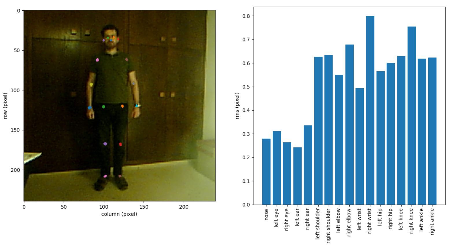
Video 1 shows an example for the RIGHT_WRIST keypoint. In the image, blue dots indicate individual pose estimation results for the 500 frames of the 5 second recording. The red dot shows the pose estimation result for the current frame and the red cursor in the plots on the right indicates the current frame in the line plots of the row coordinate and column coordinate, respectively. The orange curves in the line plots show the low-pass filtered data. The line plot on the lower right shows the residual for each frame. As an example, a threshold at 3 pixels is shown (yellow horizontal line). All residuals above this threshold are highlighted with a yellow circle. The corresponding coordinates are also highlighted with yellow circles in the camera image.

Video 1: Tracking results for keypoint RIGHT_WRIST

It can be seen that the points with high tracking errors concentrate at a specific position, where the camera perspective is such that the RIGHT_WRIST coordinate is almost identical with the RIGHT_ELBOW coordinate.

To get an impression of the lower of the lower bound of the residual, I recorded a 5 second video of a still person and computed the rms residual for the full 500 frames for each keypoint. The results are shown in figure 1. It can be seen that the typical rms value of the residual is below one pixel.

Figure 1: Tracking results for a still person

Video 2 shows an example for the LEFT_ANKLE keypoint, this time the image is slightly zoomed, as can be seen by the axes limits. Again, the points with high residual concentrate at a certain position. This time it is the upmost position of the ankle during the movement. Admittedly, the contrast between the foot and the background is very low here.

Video 2: Tracking results for keypoint LEFT_ANKLE

I think the proposed procedure is helpful to identify situations where the pose estimation precision is lower as usual. It should be possible to provide a live display of this information to the player.

Additionally to the references I made in the 'Prior art' section in the main project description, I recently found two other pieces of work that I would like to mention.

The first is [Mayuresh1611]’s paper piano that was presented in a recent hackaday.com blog post. The project uses Mediapipe's hand pose detection to create a piano experience on blank sheets of paper. I am not sure how well the implementation works for actual music making, but I must admit that the whole idea is very close to lalelu_drums.

The second is a TEDx talk given by Yago De Quay in 2012. He employs a kinect device to detect the pose of a human dancer and creates music and video projections from the data. While I still think the framerate of the kinect's pose estimation (30fps) is too slow for precise music making, I find that the talk contains many nice ideas of how to use the pose estimation technique to create an appealing live performance.

While the main target of lalelu_drums is to control percussive instruments, I would like to show a tonal example in this log entry. I chose the german lulaby "Weißt Du wie viel Sternlein stehen?" as a song that I accompany with chords triggered by gestures.

The first verse of the song is about the multitude of stars and clouds that can be seen in the sky. I chose the triggering gestures to resemble pointing at the stars or showing the moving clouds.

I would like to provide the MIDI out functionality to the backend so that I can use the drum sounds of my Roland JV-1080 sound generator. In this log entry, I explain how I setup the MIDI out and what difficulties I faced.

MIDI follows the communication protocol of a serial port with two special aspects:

• Some dedicated wiring is necessary, since the MIDI ports rely on opto-isolators.
• MIDI uses a baudrate of 31250Hz, which is not a standard serial port baudrate.

On a RaspberryPi, it is straightforward to create a MIDI output from one of the serial ports as described in this article. Since operating a serial port from python does not require a special driver, I wanted to use the same approach for my x86 based backend. So when I was selecting the backend mainboard, I carefully looked for one that provides an onboard serial port and I ended up with a MSI Z97SLI.

However, I had to learn that an RS232 output (which my mainboard provides) uses different voltage levels than the UART that a RaspberryPi has. I now use a USB-powered converter (€4,60).

But still, the communication did not work and it took me some time to figure out that even though I could set the baudrate to 31250Hz without error message, the serial port was actually operating at the next standard baudrate which is 38400Hz.

It turns out that the 16550A chipset that my mainboard uses for the serial port just does not support custom baudrates different from the default baudrates (at least I did not manage to configure it accordingly). On the RaspberryPi the MIDI baudrate of 31250Hz could be configured without difficulties from the python script opening the port.

Now I use a dedicated PCI card that provides serial ports using an AX99100 chipset (€17,95). There is a dedicated linux driver on the manufacturer's homepage that I could compile without problems ('make'). In order to permanently add the driver, I had to

• place the binary module ax99100.ko in /lib/modules/5.15.0-91-generic/kernel/drivers ('5.15.0-91-generic' being the kernel I use as returned by 'uname -r')
• add the name 'ax99100' to /etc/modules
• run 'sudo depmod'

With the driver comes a command line tool 'advanced_BR' that can be used to configure custom baudrates. I could successfully run MIDI out communication with the following configuration:

advanced_BR -d /dev/ttyF0 -b 1 -m 0 -l 250 -s 16

It configures a base clock of  125MHz (-b 1), a divisor of 250 (-m 0 -l 250) and a sampling of 16 (-s 16), yielding a nominal baudrate of 125MHz / (250 * 16) = 31250Hz.

So now, after a lot of trial-and-error, I have a serial-port-based MIDI out for ~20€, that performs very well. I still wonder, how a USB-MIDI adapter would compare to my solution in terms of linux-driver-hassle and latency / jitter.

In this log entry I present some benchmarks regarding the inference speed of the movenet model I use for human pose estimation. The benchmarks are carried out on the backend system, comprising a i5 4690K four-core CPU and GTX1660 GPU with 6GB memory.

To download the model from www.kaggle.com, search for 'movenet' in the models section, select the 'tensorflow 2' tab, select 'single-pose-thunder' from the variation drop-down menu. It offers version 4 of the pretrained model. Download the 'saved_model.pb' file and the complete 'variables' directory and place everything in a local directory.

For the benchmark I use the following code. It measures the time of the first inference, then it runs 100 inferences without measurement for warmup. The measurement is done for 2000 inferences with different random input images.

Code snippet 1: Inference benchmark

import numpy as np
import tensorflow as tf
from time import monotonic


modelPath = '/home/pi/movenet_single_pose_thunder_4'
model = tf.saved_model.load(modelPath)
movenet = model.signatures['serving_default']

# create 8-bit range random input
input = np.random.rand(1, 256, 256, 3) * 255
input = tf.cast(input, dtype=tf.int32)

start = monotonic()
out = movenet(input)
print(f'first inference time: {(monotonic() - start)}')

nWarmup = 100
for i in range(nWarmup):
    out = movenet(input)

print('starting measurement')

nMeasure = 2000
times = []

for i in range(nMeasure):
    input = np.random.rand(1, 256, 256, 3) * 255
    input = tf.cast(input, dtype=tf.int32)
    start = monotonic()
    out = movenet(input)
    times.append(monotonic() - start)
    
print(f'mean inference time: {np.mean(times)}')
print(f'min inference time: {np.min(times)}')
print(f'max inference time: {np.max(times)}')
print(f'standard deviation: {np.std(times)}')

The results can be found in the first row ('plain tensorflow') of table 1. The average inference time of 23.4ms is quite disappointing, given that I could measure 27ms already on a RaspberryPi 4 with a Google Coral AI accelerator.

Table 1: Benchmark results

In order to accelerate the inference, I used nvidias TensorRT inference optimization. The following code creates an optimized version of the model. With this optimized code, I obtained the values in the second row ('tensor rt') of table 1. The average inference time was reduced approximately by a factor of four. The optimization itself took 82 seconds.

Code snippet 2: TensorRT conversion

import numpy as np
import tensorflow as tf
from tensorflow.python.compiler.tensorrt import trt_convert as trt
from time import monotonic


start = monotonic()

inputPath = '/home/pi/movenet_single_pose_thunder_4'

conversion_params = trt.TrtConversionParams(
    precision_mode=trt.TrtPrecisionMode.FP32)
    
converter = trt.TrtGraphConverterV2(input_saved_model_dir=inputPath,
                                    conversion_params=conversion_params)
converter.convert()

def input_fn():
    inp = np.random.random_sample([1, 256, 256, 3]) * 255
    yield [tf.cast(inp, dtype=tf.int32)]

converter.build(input_fn=input_fn)

outputPath = '/home/pi/movenet_single_pose_thunder_4_tensorrt_benchmark'
converter.save(outputPath)

print(f'processing time: {monotonic() - start}')

I could reduce the average inference time further by adding the following lines to the beginning of the benchmarking script. They assign the python process to a specific core of the four-core CPU. With this change, I obtained the values in the third row ('tensor rt + cpu_affinity') of table 1.

Code snippet 3: CPU affinity

import psutil

osProcess = psutil.Process()
osProcess.cpu_affinity([2])

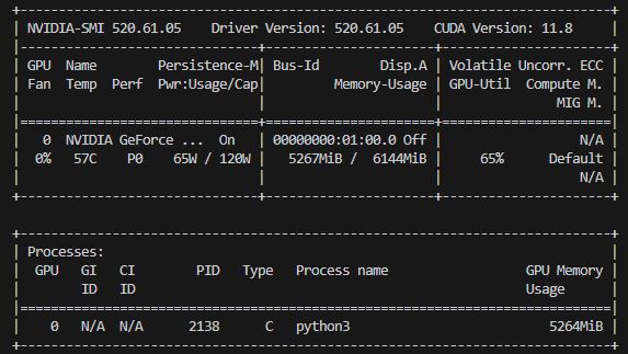
During the measurement 'tensor rt + cpu_affinity', htop shows that actually only one CPU core is used.

nvidia-smi shows that the GPU runs at half of its maximum power usage and the fan is completely off.

The results of the accelerated configuration are really satisfactory. Not only is the average inference time (3.8ms) approximately a factor of seven lower than with the Google Coral AI accelerator (27ms, RaspberryPi4), but here, the computation precision is higher (float32 instead of int8), yielding better pose estimation results (not shown here).

I also measured the inference time in the lalelu_drums application. The following graph shows the results for 1000 consecutive inferences performed for live camera images at a framerate of 100 frames per second.

It can be seen that in this environment the inference time is larger again (5ms ...6.6ms) and that there are random switches between fast and slow phases. Currently I do not have an explanation for any of the two observations. I did not yet experiment with the isolcpu setting, that I used in the RaspberryPi4 setup, though.

However, I am very happy, that I can achieve 100fps live human pose estimation with floating point precision and more-or-less realtime performance. This should be a good basis for building a low-latency musical instrument.