Project Logs

Collapse

• Edge Impulse and model in action

  kasik • 06/04/2024 at 13:47 • 0 comments

  I thought to try out person detection with Edge Impule and Neuton. Unfortunately, I didn't manage to check Neuton completely for free, thus I gave up on that idea.

  Regarding Edge Impulse - it is very intuitive to use and support is very quick and helpful. There are many tutorials available, courses by Shawn Hymel on his Youtube channel or on Coursera. There is also a book TinyML coockbook by Gian Marco Iodice - thus I will focus on results.

  
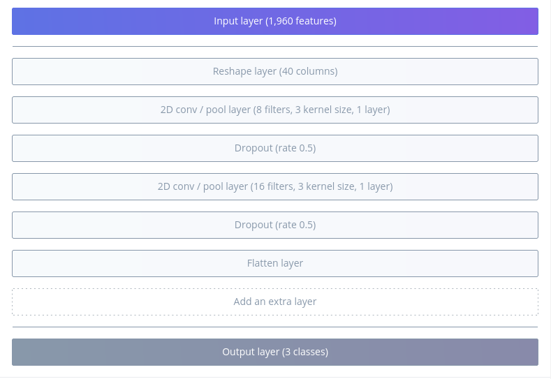
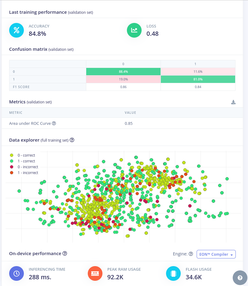
  I made a project for person_detection and used the same dataset as I did so far. What I find cool about Edge Impulse is that you can have a look at the architecture proposed and additionally you are free to make the changes.
  Training results:

  While looking at the model architecture, it is very similar to what I have been describing in previous posts. The differences lie in the hyperparameters. Interesting enough, when I copied the exact code from Edge Impulse, I didn't receive the same results.

  After the training with Edge Impulse - let's generate the code for Arduino! Obviously the code needs to be very generic, thus it is a little bit harder to follow. For easier comparison, I added the parts to check the time needed for inference and the transfer if image and the results to the PC.
  Impressive size!!!

  Let's see the execution time:
  

  Time taken by readout and data curation: 2742 ms
  Time taken by inference: 417 ms

  I noticed that in the generated code, the image retrieved is RGB (585) with resolution 160X120 and 1 fs (while I trained the model with grayscale images). Additionally, the image is only cropped to retrieve 96x96 image size. While in my code, I used grayscale, QCIF, 5fs - the image was first scaled and then cropped. I tried to modify the Edge Impulse example to increase the frame rate, but after that I stopped retrieving any images.

  And in the video - both models in action!
  

• Using bigger image

  kasik • 05/31/2024 at 14:16 • 0 comments

  I had some people asking me, why do I use images of 96x96? The full image shouldn't make that big of a difference?
  Well, actually it does. But to be able to give a quantitative answer, I had to run model training with the full image retrieved from the camera, that is 176x144 pixels.

  174x144    loss: 0.3612 - accuracy: 0.8543 - val_loss: 0.3854 - val_accuracy: 0.8390
  96x96    loss: 0.0098 - accuracy: 0.9958 - val_loss: 0.6703 - val_accuracy: 0.9280
  

      
  174x144    

  Test accuracy model: 0.8973706364631653
  Test accuracy quant: 0.897370653095844
      
  96x96    

  Test accuracy model: 0.9652247428894043
  Test accuracy quant: 0.9609838846480068
      
    c array size 174x1444 187624 compared to 66792 for 96x96 -> I don't need to add that it doesn't fit on the microcontroller!
  

• Inference on microcontroller

  kasik • 05/27/2024 at 18:44 • 0 comments

  In last episode we have successfully converted the model to be used by our microcontroller.

  In the log I have mentioned the libraries needed for Arduino. Arduino_TensorFlowLite library comes with examples, you can even find person_detection one and you will have a basic sketch prepared for you - I think it is a good start. 

  I won't go into details on the layout of the sketch and how to use the TensorFlowLite library here, as I will never do a better job than Pete Warden and Daniel Situnayake in the book "TinyML".
  Please, note that in the example person_detection in Arduino_TensorFlowLite there is uint8 quantization used:

   // Process the inference results.
    int8_t person_score = output->data.uint8[kPersonIndex];
    int8_t no_person_score = output->data.uint8[kNotAPersonIndex];

   
  And as I mentioned in the log this isn't supported (at least at the moment of writing this)

  We can treat that example as a basis for our code. In my project, I add basic image processing and then I transfer the image data together with the score via serial port to display it on my PC.
  I configured my camera to retrieve grayscale QCIF images which are 176x144 pixels. Since I trained the model using images of 96x96 pixels I need to "downsize" it. What I decided to do, is to first scale the image to 160x120 and then crop the centre to receive 96x96. Let's not forget, that the image still needs to be normalized and quantized before it can be passed to the model.

  Let's compile it and upload to the board:

  Time taken by readout and data curation: 48 ms
  Time taken by inference: 372 ms

  camera_cont_display.py is a python script (in my repo) that reads continuously from serial port, first 2 bytes is a header: label and score and then based on the WIDTH and HEIGHT I calculate the number of bytes needed for the image.

  It works!

• Converting the model

  kasik • 05/24/2024 at 13:23 • 0 comments

  In the previous logs I gathered the data, pre-procesed it, built a network, trained the network and did my best to tune the hyperparameters.

  Now it is time for the fun part -> convert the model to something understandable by my arduino and eventually deploy it on the microcontroller.
  

  Unfortunately, we won't be able to use TensorFlow on our target but rather TensorFlow lite. Before we can use it though, we need to convert the model using TensorFlow Lite Converter's Python API. It will take the model and write it back as a FlatBuffer - a space-efficient format. The converter can also apply the optimizations - like for example quantization. Model's weights and biases values are typically stored as 32-bit floats. On top of that, after normalization of my input image, the pixels values range from -1 to 1. This all leads to costly high-precision calculations. If we decide for quantization, we can reduce the precision of the weights and biases into 8-bit integers or we can go one step further - we can convert the inputs (pixel values) and outputs (prediction) as well.
  Surprisingly enough, that optimization comes with just a minimal loss in accuracy.

  # Convert the model.
  converter = tf.lite.TFLiteConverter.from_saved_model("model")
  # #quantization
  converter.optimizations = [tf.lite.Optimize.DEFAULT]
  converter.representative_dataset = representative_data_gen
  converter.target_spec.supported_ops = [tf.lite.OpsSet.TFLITE_BUILTINS_INT8]
  converter.inference_input_type = tf.int8
  converter.inference_output_type = tf.int8
  tflite_model = converter.convert()

  Note, that only int8 is available now in TensorFlow Lite (even though uint8 is available in API) - it took me quite some time to understand that it is not a problem of my code.

  In the above snippet, you can see a representative_dataset - it is a dataset that would represent the full range of possible input values. Even though I have come across many tutorials, it still caused me some troubles. Mainly because the API expects the image to be float32 (even if for training you used a grayscale image in range from -128 to 127 and type of int8).
  

  def representative_data_gen():
    for file in os.listdir('representative'):
      # open, resize, convert to numpy array
      image = cv2.imread(os.path.join('representative',file), 0)
      image = cv2.resize(image, (IMG_WIDTH, IMG_HEIGHT))
      image = image.astype(np.float32)
      # image -=128
      image = image/127.5 -1
      image = (np.expand_dims(image, 0))
      image = (np.expand_dims(image, 3))
      yield [image] 
  
  
  

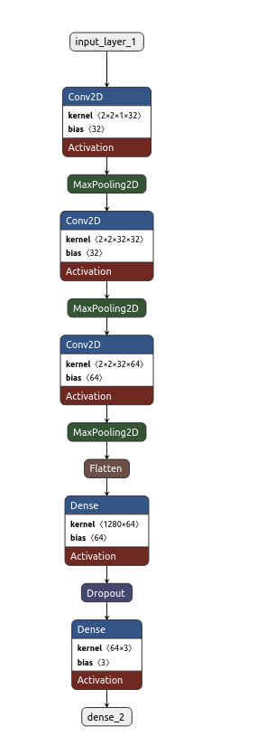
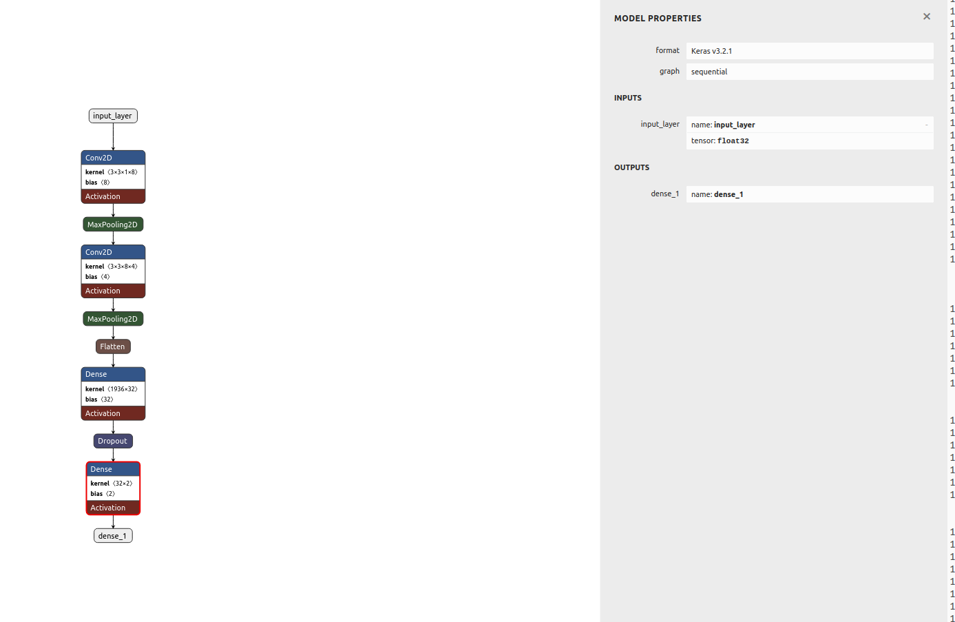
  Let's see both models architecture using Netron. First basic model:

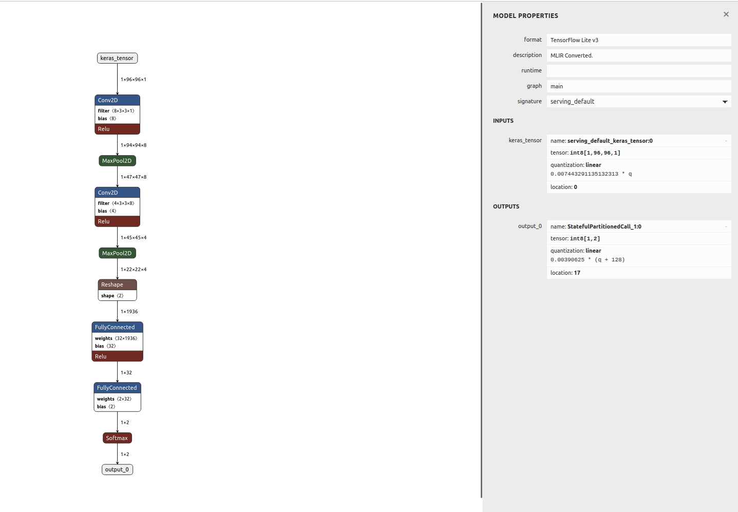
  and quantized one:
  

  I wanted to make sure that the conversion went smoothly and the model still works before deploying anything to microcontroller. For that I would make predictions with both models - the initial one and the converted and quantized one. It is slighlty more complex to use the Tensorflow Lite model as you can see in the snippet below. Additionally, we need to remember to quantize the input image with retrieved scale and zero point values from the model.
  

  # Load the TFLite model in TFLite Interpreter
  interpreter = tf.lite.Interpreter(tflite_file_path)
  
  # Load TFLite model and allocate tensors.
  interpreter = tf.lite.Interpreter(model_content=tflite_model)
  interpreter.allocate_tensors()
  
  # Get input quantization parameters.
  input_quant = input_details[0]['quantization_parameters']
  input_scale = input_quant['scales'][0]
  input_zero_point = input_quant['zero_points'][0]
  
  #quantize input image
  input_value = (test_image/ input_scale) + input_zero_point
  input_value = tf.cast(input_value, dtype=tf.int8)
  interpreter.set_tensor(input_details[0]['index'], input_value)
  
  
  # run the inference
  interpreter.invoke()

  Results of comparison:

  Test accuracy model: 0.9607046246528625
  Test accuracy quant: 0.9363143631436315
  Basic model is 782477 bytes
  Quantized model is 66752 bytes

   
  
  The last thing that needs to be done is converting the model to C file. In Linux we can just use xxd tool to achieve that:

  def convert_to_c_array...

  Read more »

• Normalization

  kasik • 05/19/2024 at 11:31 • 0 comments

  I realized I haven't mentioned normalization so far. Usually it is common in machine learning problems to pre-process the data as a first step, before training. This often means to zero-mean (center) the data and normalize by standard deviation. Zero-centering helps to reduce the effect of biases in the network. Since the network is learning from data that has been centered around zero, it is less likely to develop biases towards certain features or patterns in the data. The goal for normalization is to ensure that all features are within the same range thus contribute equally.
  

  An interesting technique is batch normalization - where we try to keep the activations as a Gaussian function - it normalizes the input to each of the layers. Batch normalization enables the use of much higher learning rates during training - as normalizing the inputs prevents them from becoming too large or small. This directly helps to prevent exploding and vanishing gradient issues, often faced with high learning rates and complex architectures. Batch normalization can be added as a layer in the network.
  

  I must admit this somehow wasn't very intuitive to me regarding my current project - as I am working with grayscale images with pixel values ranging from 0 to 255. Yet, the results speak for themselves.
  when normalization used -> validation loss got  0.3 and validation loss got close to 0.9!

  I run the above multiple times to ensure I wasn't just lucky with the initializations.
  

• Visualizing CNN

  kasik • 05/17/2024 at 14:25 • 0 comments

  Neural Networks can be often viewed as a kind of black boxes - with a lot of computation happening behind the scenes. I thought it would be really interesting to be able to somehow visualize their work. 

  There are various ways to visualize what CNNs do. Personally, I find visualizing feature maps and regions that are most important for the network, particularly interesting.
  Seeing the feature maps can show us the internal representation of the input the model has in a specific location - which features are found and focused on by the CNN.

  It is very easy to see visualize them in python, we can  simply take the first convolution layer and make a prediction with that subset of network. The result will give us the 8 feature maps :

  # redefine model to output right after the first hidden layer
  model = Model(inputs=probability_model.inputs, outputs=probability_model.layers[1].output)
  model.summary()
  
  # get feature map for first hidden layer
  feature_maps = model.predict(test_image)
  # plot all 8 maps in an 2x4 squares
  r = 2
  c = 4
  ix = 1
  for _ in range(r):
  	for _ in range(c):
  		# specify subplot and turn of axis
  		ax = plt.subplot(r, c, ix)
  		ax.set_xticks([])
  		ax.set_yticks([])
  		# plot filter channel in grayscale
  		plt.imshow(feature_maps[0, :, :, ix-1], cmap='gray')
  		ix += 1
  # show the figure
  plt.show()

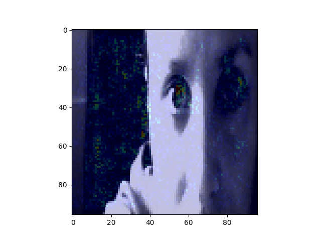
  Another interesting way to show what is going on with our model is something called saliency map - with this technique we can see where our network focuses thus we can understand better the decision process.It is most common to visualize the saliency maps as the heatmap overlayed on the image of interest. There are various ways to compute the saliency map, there are even several gradient-based approaches - where the gradient of prediction with respect to input features is calculated. Symonian et al. were the first (in 2013) to propose a method that uses backpropagation to calculate the gradient of the loss function for the class we are interested in with respect to the input pixels. An example (I based mine on other available ) is in the script and here are some results:

• Data augmentation

  kasik • 05/05/2024 at 14:29 • 0 comments

  I mentioned data augmentation already in a few logs, so I thought I will write about it briefly. Data augmentation is used to enhance the training set by creating additional training data based on existing data (in our case: images). It can be modifying the existing ones or even using generative AI to create new ones! I will mention the first technique as I didn't have yet the chance to dive into generative AI.

  A few examples:
  

  • adding noise
  • geometric transformation - cropping, rotating, zooming

  NOTE: The biases in the original dataset persist in the augmented data.

  There are at least 2 ways readily available for data augmentation. One would be to use keras.Sequential() - yes, the same one used to build the model. It turns out that there are also augmentation layers that can be added. Moreover, the preprocessing layers can be part of the model (note: the data augmentation is inactive during the testing phase. Those layers will only work for Model.fit, not for Model.evaluate or Model.predict) or the preprocessing layers can be applied to the dataset. Another available method is to use tf.image - which gives you more control. Official simple and clear example for both.
  

  Or, perhaps, just for fun you can create your own preprocessing. In my repository you can find data_augmentation.py - where I implemented some transformations of the images. It is a very simple script, which creates 8 extra images out of 1 - it flips, rotates and adds noise.
  All of the nine images are saved in a new directory, in that case called 'output'.

  A comparison of the training results with and without using augmentation:

  I had a chat recently about a medical device (SaMD - Software as a Medical Device) that was trained on the dataset of 7 images. Much to my surprise I understood that it was working quite well! Don't worry, it was only guiding the medical personnel ;) I would love to have a chat with the developers to understand whether they used transfer learning/ data augmentation or perhaps even a different algorithm?

• Useful Metrics

  kasik • 04/30/2024 at 09:58 • 0 comments

  Today a few notes on useful metrics. In one of the previous logs I mentioned looking at accuracy and loss, but of course the topic is more complex. Sometimes accuracy may even be misleading. 

  Let's imagine that we have a naive classifier - a classification algorithm with no logic or rather with minimum effort and data manipulation to prepare a forecast. We want to model anomaly detection, with 0 for no anomaly and 1 for anomaly detected. We can use for example a method called Uniformly Random Guess: that predicts 0 or 1 with equal probability. Or even better - an algorithm that always outputs 0. With a low anomaly rate, we can get the accuracy of our algorithm even 100% and have an impression that we did an excellent job.
  

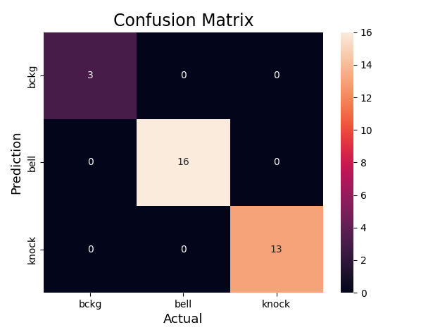
  A nice tool to consider is a confusion matrix - a table where we have predicted labels and actual labels with scores for each, for example:

  It is very easy to create and display the confusion matrix in python using sklearn.metrics:
  

      # Compute confusion matrix
      cm = confusion_matrix(y_val, y_pred)
  
      sns.heatmap(cm,
                  annot=True,
                  fmt='g',
                  xticklabels=['Person', 'Not person'],
                  yticklabels=['Person', 'Not person'])
      plt.ylabel('Prediction', fontsize=13)
      plt.xlabel('Actual', fontsize=13)
      plt.title('Confusion Matrix', fontsize=17)
      plt.show()

  
  
  Useful terms related with confusion matrix:
      True Positive (TP): Values that are actually positive and predicted positive.
      False Positive (FP): Values that are actually negative but predicted positive.
      False Negative (FN): Values that are actually positive but predicted negative.
      True Negative (TN): Values that are actually negative and predicted negative.

  With the use of the above, we can calculate the following:
  Precision
  Out of all the positive predicted, what percentage is truly positive.

  Precision = True Positive/Predicted Positive

  Recall
  Out of the actual positive, what percentage are predicted properly.  
  Recall = True Positive/Actual Positive

  It is very common to calculate F1 score, which is used to measure test accuracy. It is a weighted average of the precision and recall. When F1 score is 1 it’s best and on 0 it’s worst.

      F1 = 2 * (precision * recall) / (precision + recall)
     
  

  Note, that the above are calculated for the target class and not for the full system.

  And as always, we need to have our particular problem in mind, in some cases the occurrences of False Negatives have more severe consequences then False Positives (for example cancer detection). Which means we may need to consider some weights in the calculation of metrics or maybe even choose different ones.

• Overfitting

  kasik • 04/29/2024 at 09:23 • 0 comments

  It seems I haven't been here for a while, fear not - the project continues! Due to some other projects, I was forced to upgrade my Linux distribution, thus most of the packages got updated as well. I must admit, It took me an hour or two to fix the project due to changes in the libs. Now I am using Keras version 3.2.1.

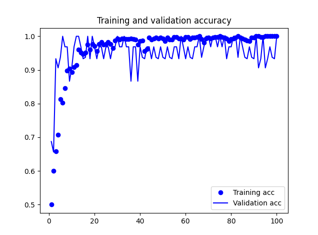
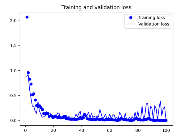
  I wanted to come back to the topic of overfitting, which can cause many troubles when working on a model. Very often, while observing the training progress - we may see a beautiful curve of training and  accuracy that reaches 1 very quickly and stays there. At the same time - the training loss gets very close to 0. Such graphs may lead to a false impression that we have created an excellent neural network. 

  Unfortunately that is too good to be true. If we look at the validation graphs instead, it doesn't seem so great anymore - the accuracy and loss lag way behind and achieve worse performance.
  What actually happens is that the neural network becomes too specialized, learns the training set too well, that it fails to generalize on the unseen data.
  And that is overfitting in a nutshell. There are various ways to fight that.

  1. Use more data!
  Sounds easy enough yet not always feasible. It shouldn't come as a surprise that there are ways to overcome that as well, such as data augmentation (log post coming soon) or even transfer learning, where a pretrained model is used (log post coming soon).
  As a note - random shuffling the data order has a positive effect as well.

  2. Model ensembles
  Sounds strange, doesn't it? Model ensembles means using several neural networks with different architectures. However, it is quite complex and computationally expensive.

  3. Regularization
  I used this term already a few times - this is a set of techniques that penalizes the complexity of the model. Its goal is to add some stochasticity during training. It can mean for example adding some extra terms during the loss calculation or early stopping - which means stopping learning process when the validation loss doesn't decrease anymore.
  A technique that I find interesting is a dropout - where the activations from certain neurons are set to 0. Interesting enough - this can be applied to neurons in fully connected layers or convolution layers - where a full feature map is dropped. This means that temporarily new architectures are created out of the parent network. The nodes are dropped by a dropout probability of p (for the hidden layers, the greater the drop probability the more sparse the model, where 0.5 is the most optimised probability). Note that this differs with every forward pass - meaning with each forward pass it is calculated which nodes to drop. With dropout we force the neural network to learn more robust features and not to rely on specific clues.  As an extra note - dropout is applied only during training and not during predictions.

  On the graphs below you can se the effect of adding a dropout: - the the validation loss follows the curve of training loss; the training accuracy doesn't reach immediately 1 and validation accuracy follows the training one.
  

  In my project I use dropout on fully connected layers, I will further increase the dataset, use data augmentation, try out transfer learning.

• Training

  kasik • 04/01/2024 at 11:32 • 0 comments

  It is finally time to train the model that I described in the previous log - the script is available in my repository and is called person_detection.py
  First I need to load the data and make sure the images are 96x96 pixels grayscale. We will need to use int8 for the input on the microcontroller (uint8 is not accepted), hence I also convert the images to that range. I created a module dataset.py for the purpose of loading data as I will be reading images also in another script. I always like to check my dataset so, I choose a picture for display:
  
  

  plt.imshow(images[1], cmap='gray', vmin= -128, vmax=127)

  Then I split the data to use 60% as training set, 20% as validation set and 20% as test set . Note that train_test_split method can shuffle the data.
  

      #split images to train, validation and test
      X_train, x_test, Y_train, y_test = train_test_split(np.array(images), np.array(labels), test_size= 0.2)
      x_train, x_val, y_train, y_val = train_test_split(X_train, Y_train, test_size = 0.25) 
   

  Validation set is used to check the accuracy of our model during the training. Next step is to create the model (as per last log) and finally - time to train:
  

    # Fit model on training data
      history = model.fit(x_train, y_train, epochs=EPOCHS, validation_data=(x_val, y_val))

   
      
  Here we need to choose batch size end epochs. Batch size specifies how many pieces of training data to feed into the network before measuring its accuracy and updating its weights and biases. Big batch size leads to less accurate models. However, it seems that the models trained with large batch sizes tend to become dataset specialized thus they are more likely to overfit. Too small batch size on the other hand results in a very long computation time. Small batch size means that we will need to calculate the parameters more frequently - hence increased training time.
  Regarding epochs - this parameter specifies the number of times the network will be retrained. The intuition would be - the more the better - however, this would affect not only the computation time, but also it turns out that some networks may start to overfit.

  And voila! We can observe the training progress.

  When the training is done, I want to observe the basic metrics:

      # Extract accuracy and loss values (in list form) from the history
      acc = history.history['accuracy']
      val_acc = history.history['val_accuracy']
      loss = history.history['loss']
      val_loss = history.history['val_loss']
  
      # Create a list of epoch numbers
      epochs = range(1, len(acc) + 1)
  
      # Plot training and validation loss values over time
      plt.figure()
      plt.plot(epochs, loss, color='blue', marker='.', label='Training loss')
      plt.plot(epochs, val_loss, color='orange', marker='.', label='Validation loss')
      plt.title('Training and validation loss')
      plt.legend()
  
      # Plot training and validation accuracies over time
      plt.figure()
      plt.plot(epochs, acc, color='blue', marker='.', label='Training acc')
      plt.plot(epochs, val_acc, color='orange', marker='.', label='Validation acc')
      plt.title('Training and validation accuracy')
      plt.legend()
      plt.show()

  Obviously we would like that validation accuracy follows closely accuracy on the training set, similarly the validation loss shall follow loss on the training set. Of course the validation set will perform worse, but we don't want them to fall too far apart.

  After that, let's try out our training set.
  
  

      # Evaluate neural network performance
      score = model.evaluate(x_test,  y_test, verbose=2)

   
     
  Just like that I have my first model trained - however, now it is time to play with basic hyperparameters and try to achieve better results.

  Happy playing!

View all 15 project logs