TinyML meets dog training

Next steps:

• my initial prototyping hardware platform has a microphone and camera, however the camera is very basic and having in mind future features of the device, I thought to research something else - and I found Seeed Studio XIAO ESP32S3
• I gave it a try in the recent days - I made a model for a camera and then I made a model for the Keyword Spotting (separately) - still some work to be done to improve. Next step will be to make a code for both models at the same time
• communicate with another feeder
• design my own feeder
• I would love to put it on some crowdfunding

Having both models working in the decent way I was eager to try it out. In the video below, you can see the feeder being triggered upon a knock sound.

The plan is to build a custom feeder, however it will still take some time for me to design it. Additionally, I thought my device could be useful for someone already having a feeder. Plus, let's face it - this part was fun :) So we figured out a way how to communicate with a Trixie Activity Dog Trainer feeder as the most popular and affordable one.

I use nrf24l01 for the communication with the feeder.

I haven't been here for a while but it doesn't mean there was no progress with my project, just not much time to document everything in nice articles. I would love to take part in the contest 2025 Pet Chacks Challenge so I will focus now on description and hopefully soon I will come back here with playing around and with more tutorial style articles.

The last time I made a decent face recognition model both from scratch and with help of Edge Impulse.
In this project I will need to use  two models - image recognition and keyword spotting (not to mix with sensor fusion). My arduino nano 33 ble sense has also a microphone, this is why it was selected in the first place - but apparently mine is not working (took me a while to accept it is not me doing sth wrong).

I went on to search for some different hardware - i selected Seed Studio XIAO nRF52840 as both use the same microcontroller.

Ok, now to keyword spotting. For my application I want to be able to react upon the sound of a knock and doorbell. The first step is data gathering - I used mainly FSD50K datasets, where I searched for the variations of: knocking and doorbell sounds. My third class - background had to be robust thus I tried to search for everyday house life sounds. I also made sure to include dog barking (I found even knocking and doorbell sounds with barking) and the sound of dog walking on the floor.

Unfortunately with sounds we cannot go directly to building model as it was with the images - we need to perform some processing first. First step is to ensure that all my data is 1 second long with 16kHz sampling. Next: build a spectrogram which can be considered an audio signal's image representation. To achieve that I ran FFT on every 30ms sample window with a step of 20ms (thus 10ms overlap)

A spectrogram generated this way is not ideal for voice speech recognition because it does not highlight the relevant features effectively. The spectrogram is adjusted to better align with how humans perceive frequencies and loudness on a logarithmic scale rather than a linear one. The adjustments are as follows:

•     Frequency scaling (Hz) to Mel scale: The Mel scale filter bank remaps frequencies to enhance their distinguishability and to make them appear equidistant to the human ear.
•     Amplitude scaling using the decibel (dB) scale: Since humans perceive amplitude logarithmically (similar to how we perceive frequencies), scaling the amplitudes with the dB scale better reflects this perception.

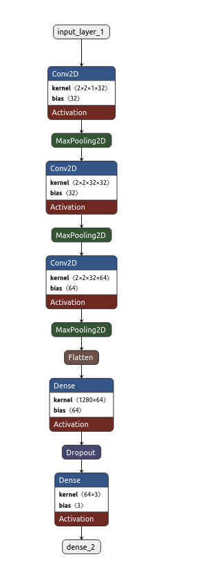
Time to build the model! Visualization below done with Netron,

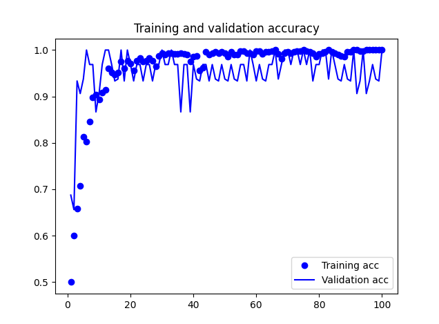
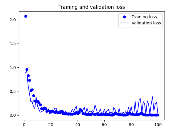
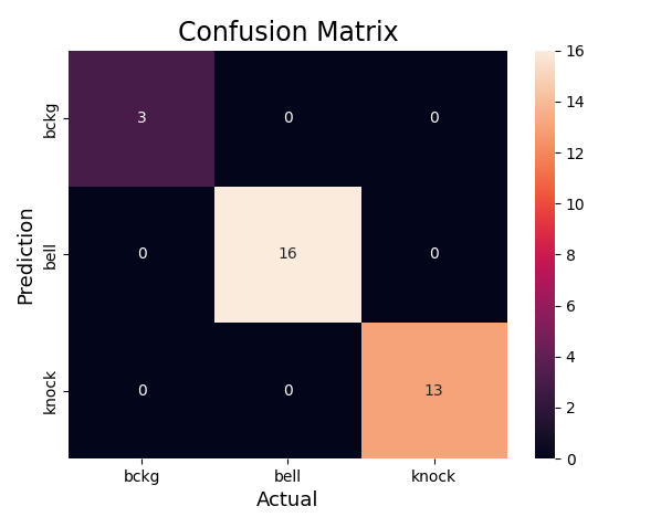
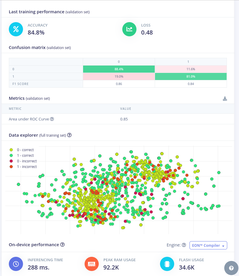
And below training results:

 Accuracy of quantized model: 0.9861809045226131

I did the same with Edge Impulse:

Now it's time for the deployment.

Both models did well during tests on the target. However, both struggled with false positives - for example putting a book/mug down was often recognised as knocking. However, I must say it is a fair mistake. There is still some work to be done here, but I believe it is good enough to continue.

I thought to try out person detection with Edge Impule and Neuton. Unfortunately, I didn't manage to check Neuton completely for free, thus I gave up on that idea.

Regarding Edge Impulse - it is very intuitive to use and support is very quick and helpful. There are many tutorials available, courses by Shawn Hymel on his Youtube channel or on Coursera. There is also a book TinyML coockbook by Gian Marco Iodice - thus I will focus on results.

I made a project for person_detection and used the same dataset as I did so far. What I find cool about Edge Impulse is that you can have a look at the architecture proposed and additionally you are free to make the changes.
Training results:

While looking at the model architecture, it is very similar to what I have been describing in previous posts. The differences lie in the hyperparameters. Interesting enough, when I copied the exact code from Edge Impulse, I didn't receive the same results.

After the training with Edge Impulse - let's generate the code for Arduino! Obviously the code needs to be very generic, thus it is a little bit harder to follow. For easier comparison, I added the parts to check the time needed for inference and the transfer if image and the results to the PC.
Impressive size!!!

Let's see the execution time:

Time taken by readout and data curation: 2742 ms
Time taken by inference: 417 ms

I noticed that in the generated code, the image retrieved is RGB (585) with resolution 160X120 and 1 fs (while I trained the model with grayscale images). Additionally, the image is only cropped to retrieve 96x96 image size. While in my code, I used grayscale, QCIF, 5fs - the image was first scaled and then cropped. I tried to modify the Edge Impulse example to increase the frame rate, but after that I stopped retrieving any images.

And in the video - both models in action!

I had some people asking me, why do I use images of 96x96? The full image shouldn't make that big of a difference?
Well, actually it does. But to be able to give a quantitative answer, I had to run model training with the full image retrieved from the camera, that is 176x144 pixels.

174x144    loss: 0.3612 - accuracy: 0.8543 - val_loss: 0.3854 - val_accuracy: 0.8390
96x96    loss: 0.0098 - accuracy: 0.9958 - val_loss: 0.6703 - val_accuracy: 0.9280

    
174x144    

Test accuracy model: 0.8973706364631653
Test accuracy quant: 0.897370653095844
    
96x96    

Test accuracy model: 0.9652247428894043
Test accuracy quant: 0.9609838846480068
    
  c array size 174x1444 187624 compared to 66792 for 96x96 -> I don't need to add that it doesn't fit on the microcontroller!

In last episode we have successfully converted the model to be used by our microcontroller.

In the log I have mentioned the libraries needed for Arduino. Arduino_TensorFlowLite library comes with examples, you can even find person_detection one and you will have a basic sketch prepared for you - I think it is a good start. 

I won't go into details on the layout of the sketch and how to use the TensorFlowLite library here, as I will never do a better job than Pete Warden and Daniel Situnayake in the book "TinyML".
Please, note that in the example person_detection in Arduino_TensorFlowLite there is uint8 quantization used:

 // Process the inference results.
  int8_t person_score = output->data.uint8[kPersonIndex];
  int8_t no_person_score = output->data.uint8[kNotAPersonIndex];

 
And as I mentioned in the log this isn't supported (at least at the moment of writing this)

We can treat that example as a basis for our code. In my project, I add basic image processing and then I transfer the image data together with the score via serial port to display it on my PC.
I configured my camera to retrieve grayscale QCIF images which are 176x144 pixels. Since I trained the model using images of 96x96 pixels I need to "downsize" it. What I decided to do, is to first scale the image to 160x120 and then crop the centre to receive 96x96. Let's not forget, that the image still needs to be normalized and quantized before it can be passed to the model.

Let's compile it and upload to the board:

Time taken by readout and data curation: 48 ms
Time taken by inference: 372 ms

camera_cont_display.py is a python script (in my repo) that reads continuously from serial port, first 2 bytes is a header: label and score and then based on the WIDTH and HEIGHT I calculate the number of bytes needed for the image.

It works!

In the previous logs I gathered the data, pre-procesed it, built a network, trained the network and did my best to tune the hyperparameters.

Now it is time for the fun part -> convert the model to something understandable by my arduino and eventually deploy it on the microcontroller.

Unfortunately, we won't be able to use TensorFlow on our target but rather TensorFlow lite. Before we can use it though, we need to convert the model using TensorFlow Lite Converter's Python API. It will take the model and write it back as a FlatBuffer - a space-efficient format. The converter can also apply the optimizations - like for example quantization. Model's weights and biases values are typically stored as 32-bit floats. On top of that, after normalization of my input image, the pixels values range from -1 to 1. This all leads to costly high-precision calculations. If we decide for quantization, we can reduce the precision of the weights and biases into 8-bit integers or we can go one step further - we can convert the inputs (pixel values) and outputs (prediction) as well.
Surprisingly enough, that optimization comes with just a minimal loss in accuracy.

# Convert the model.
converter = tf.lite.TFLiteConverter.from_saved_model("model")
# #quantization
converter.optimizations = [tf.lite.Optimize.DEFAULT]
converter.representative_dataset = representative_data_gen
converter.target_spec.supported_ops = [tf.lite.OpsSet.TFLITE_BUILTINS_INT8]
converter.inference_input_type = tf.int8
converter.inference_output_type = tf.int8
tflite_model = converter.convert()

Note, that only int8 is available now in TensorFlow Lite (even though uint8 is available in API) - it took me quite some time to understand that it is not a problem of my code.

In the above snippet, you can see a representative_dataset - it is a dataset that would represent the full range of possible input values. Even though I have come across many tutorials, it still caused me some troubles. Mainly because the API expects the image to be float32 (even if for training you used a grayscale image in range from -128 to 127 and type of int8).

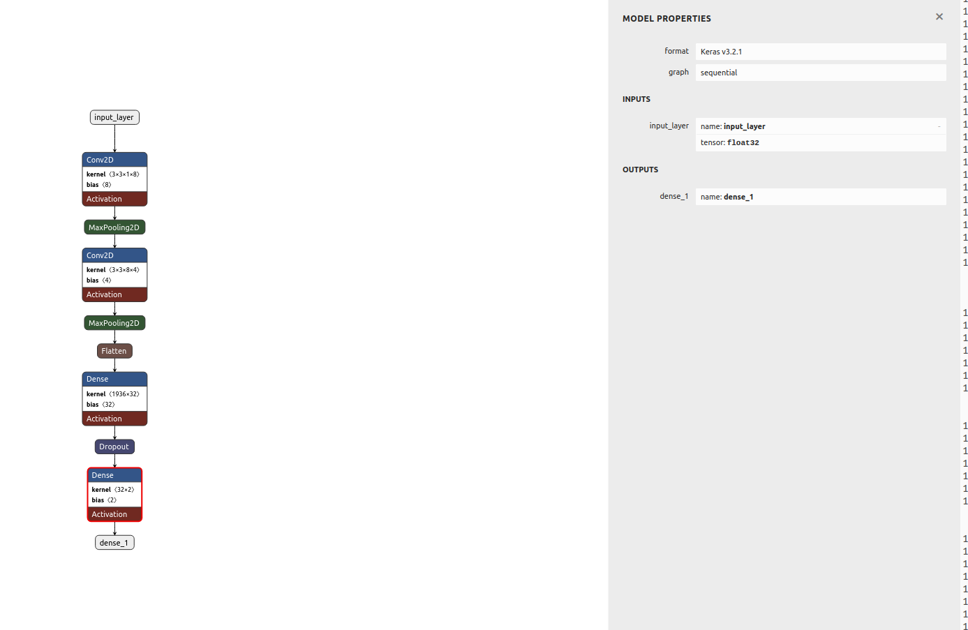
def representative_data_gen():
  for file in os.listdir('representative'):
    # open, resize, convert to numpy array
    image = cv2.imread(os.path.join('representative',file), 0)
    image = cv2.resize(image, (IMG_WIDTH, IMG_HEIGHT))
    image = image.astype(np.float32)
    # image -=128
    image = image/127.5 -1
    image = (np.expand_dims(image, 0))
    image = (np.expand_dims(image, 3))
    yield [image] 

Let's see both models architecture using Netron. First basic model:

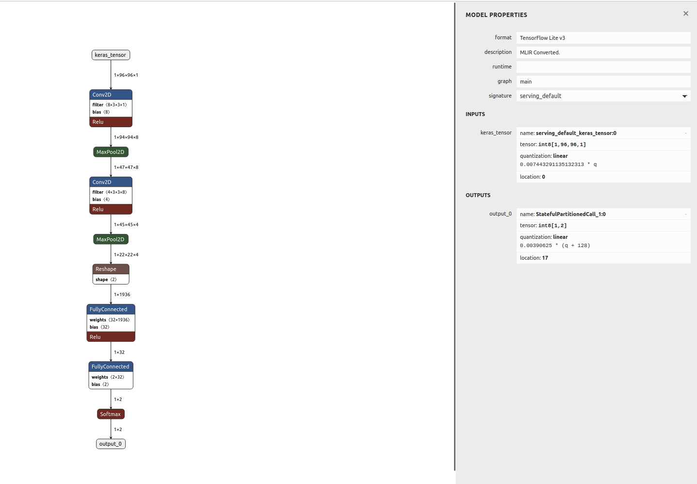
and quantized one:

I wanted to make sure that the conversion went smoothly and the model still works before deploying anything to microcontroller. For that I would make predictions with both models - the initial one and the converted and quantized one. It is slighlty more complex to use the Tensorflow Lite model as you can see in the snippet below. Additionally, we need to remember to quantize the input image with retrieved scale and zero point values from the model.

# Load the TFLite model in TFLite Interpreter
interpreter = tf.lite.Interpreter(tflite_file_path)

# Load TFLite model and allocate tensors.
interpreter = tf.lite.Interpreter(model_content=tflite_model)
interpreter.allocate_tensors()

# Get input quantization parameters.
input_quant = input_details[0]['quantization_parameters']
input_scale = input_quant['scales'][0]
input_zero_point = input_quant['zero_points'][0]

#quantize input image
input_value = (test_image/ input_scale) + input_zero_point
input_value = tf.cast(input_value, dtype=tf.int8)
interpreter.set_tensor(input_details[0]['index'], input_value)


# run the inference
interpreter.invoke()

Results of comparison:

Test accuracy model: 0.9607046246528625
Test accuracy quant: 0.9363143631436315
Basic model is 782477 bytes
Quantized model is 66752 bytes

 

The last thing that needs to be done is converting the model to C file. In Linux we can just use xxd tool to achieve that:

def convert_to_c_array():
  """ Converts the TFLite model to C array"""
  os.system('xxd -i  ' + tflite_file_path + ' > ' + c_array_model_fname)
  print("C array model created " + c_array_model_fname)

 

Et voila!

I realized I haven't mentioned normalization so far. Usually it is common in machine learning problems to pre-process the data as a first step, before training. This often means to zero-mean (center) the data and normalize by standard deviation. Zero-centering helps to reduce the effect of biases in the network. Since the network is learning from data that has been centered around zero, it is less likely to develop biases towards certain features or patterns in the data. The goal for normalization is to ensure that all features are within the same range thus contribute equally.

An interesting technique is batch normalization - where we try to keep the activations as a Gaussian function - it normalizes the input to each of the layers. Batch normalization enables the use of much higher learning rates during training - as normalizing the inputs prevents them from becoming too large or small. This directly helps to prevent exploding and vanishing gradient issues, often faced with high learning rates and complex architectures. Batch normalization can be added as a layer in the network.

I must admit this somehow wasn't very intuitive to me regarding my current project - as I am working with grayscale images with pixel values ranging from 0 to 255. Yet, the results speak for themselves.
when normalization used -> validation loss got  0.3 and validation loss got close to 0.9!

I run the above multiple times to ensure I wasn't just lucky with the initializations.

Neural Networks can be often viewed as a kind of black boxes - with a lot of computation happening behind the scenes. I thought it would be really interesting to be able to somehow visualize their work. 

There are various ways to visualize what CNNs do. Personally, I find visualizing feature maps and regions that are most important for the network, particularly interesting.
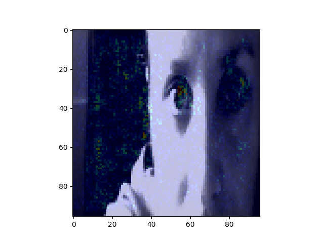
Seeing the feature maps can show us the internal representation of the input the model has in a specific location - which features are found and focused on by the CNN.

It is very easy to see visualize them in python, we can  simply take the first convolution layer and make a prediction with that subset of network. The result will give us the 8 feature maps :

# redefine model to output right after the first hidden layer
model = Model(inputs=probability_model.inputs, outputs=probability_model.layers[1].output)
model.summary()

# get feature map for first hidden layer
feature_maps = model.predict(test_image)
# plot all 8 maps in an 2x4 squares
r = 2
c = 4
ix = 1
for _ in range(r):
	for _ in range(c):
		# specify subplot and turn of axis
		ax = plt.subplot(r, c, ix)
		ax.set_xticks([])
		ax.set_yticks([])
		# plot filter channel in grayscale
		plt.imshow(feature_maps[0, :, :, ix-1], cmap='gray')
		ix += 1
# show the figure
plt.show()

Another interesting way to show what is going on with our model is something called saliency map - with this technique we can see where our network focuses thus we can understand better the decision process.It is most common to visualize the saliency maps as the heatmap overlayed on the image of interest. There are various ways to compute the saliency map, there are even several gradient-based approaches - where the gradient of prediction with respect to input features is calculated. Symonian et al. were the first (in 2013) to propose a method that uses backpropagation to calculate the gradient of the loss function for the class we are interested in with respect to the input pixels. An example (I based mine on other available ) is in the script and here are some results: