Where we were. The last log designed JASPER around a single concave variable-line-spacing (VLS) grating that disperses and focuses 500–1000 nm onto a linear CCD. That grating was an ideal: a custom groove pattern that exists only in our model. A two-beam holographic exposure could write it — the repo now includes that check (recording_optimize_sim.py: a 488 nm exposure matches the fitted grooves' resolution to within 0.02 nm) — but it is not a part anyone sells, and a custom holographic master is out of reach for a small open project. A spectrometer you can't source isn't a design, it's a study.

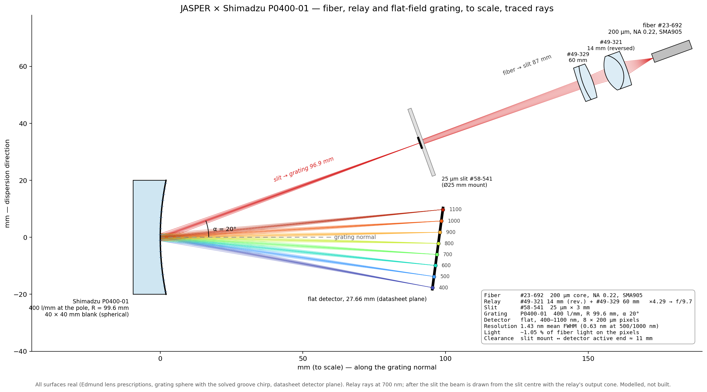
This log is the practical version. Every optical part is a catalog item:

• Grating: Shimadzu P0400-01 flat-field concave grating — 400 l/mm, 400–1100 nm, full mount published.
• Fiber: Edmund #23-692, 200 µm core, NA 0.22, VIS-NIR, SMA905.
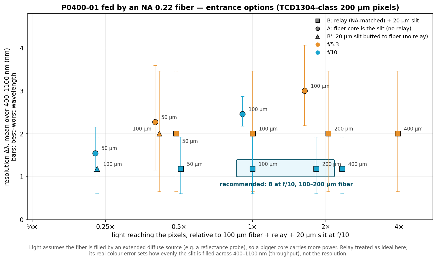
• Relay: Edmund #49-321 (14 mm) + #49-329 (60 mm) achromats, ×4.3 — turns the fiber's NA 0.22 into ~f/10 at the grating.
• Slit: Edmund #58-541, 25 µm × 3 mm.
• Detector: TCD1304-class linear CCD, 8 × 200 µm pixels, on the datasheet's detector plane.

The one unknown: the grooves. Shimadzu publishes the mount but not the groove pattern — the P0400-01 is an aberration-corrected holographic grating whose chirp is proprietary. So we reconstructed it from the datasheet. The groove density across the blank is

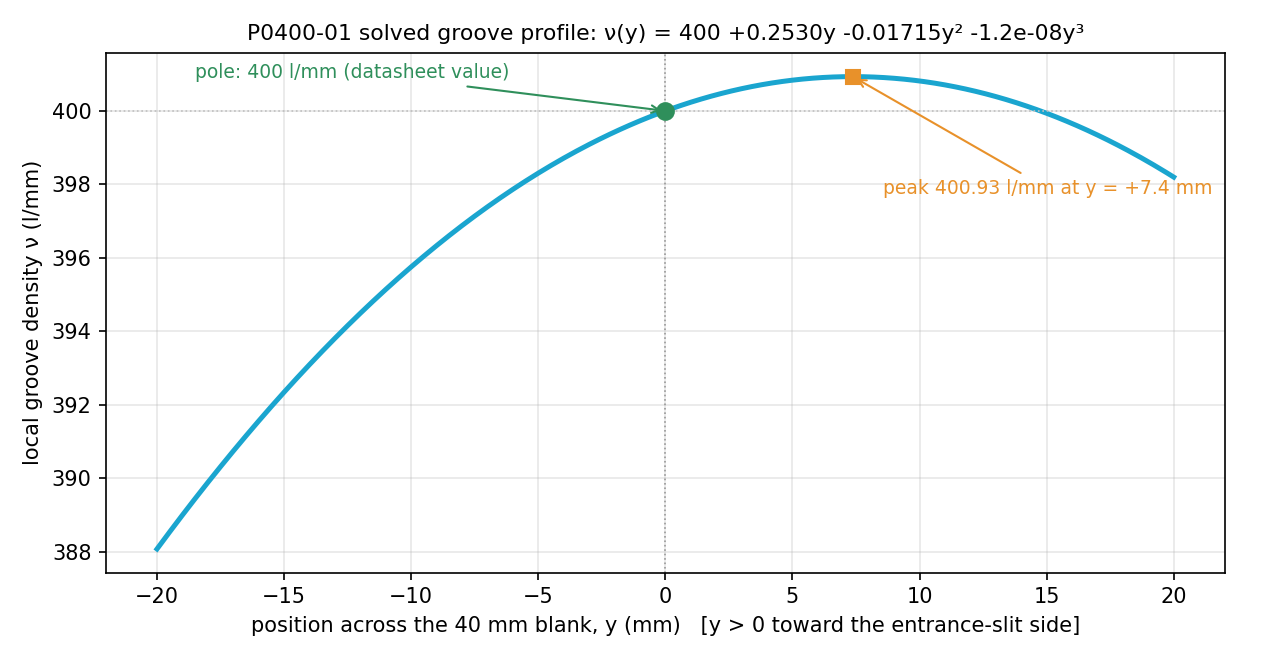
nu(y) = 400 + C1*y + C2*y^2 + C3*y^3      (lines/mm, y in mm from the grating centre)

and here is how each piece is pinned down:

1. 400 l/mm is at the centre. The grating equation with 400 l/mm at the pole gives diffraction angles of −10.49° (400 nm) and +5.62° (1100 nm) — exactly the datasheet's. If 400 were at either edge of the blank, the 1100 nm angle would miss by 0.12° or 0.76°, and the datasheet quotes it to 0.01°. That pins the centre density to 400 ± 0.16 l/mm.
2. The detector is one flat tilted plane. The datasheet's two exit distances (97.1 mm at 400 nm, 99.5 mm at 1100 nm) are the two ends of a single flat detector, which the datasheet also gives directly: r′ᵢ = 96.9 mm from the grating, normal at βᵢ = −7.51°. All four printed numbers agree for r′ᵢ = 96.92–96.95 mm; we use 96.93.
3. The radius of curvature comes from the blank. It isn't printed, but the blank is 9.5 mm thick at the centre and 13.6 mm at the corners (28.3 mm out): R = (h² + s²)/2s = 99.61 mm. A free fit gives 100.00 mm and the classical focus condition 100.29 mm — three estimates within 0.7 %.
4. What each coefficient does. C1 corrects defocus: the defocus term becomes F20 = cos²α/r − cosα/R + cos²β/r′ − cosβ/R + λ·C1, so defocus vanishes at a wavelength when C1 = −F20,geom/λ. C2 corrects coma. C3 would correct the next order.
5. Solve. With the centre density, detector plane and radius fixed, only C1–C3 are unknown. Ray tracing through the exact surface onto the fixed plane and minimising the spot size across 400–1100 nm gives C1 = +0.253 l/mm², C2 = −0.0172 l/mm³, C3 ≈ 0. Two independent checks agree: fitting C1 for a single wavelength in the ray tracer matches the analytic defocus condition to within 0.001 at all eight wavelengths (e.g. 0.300 vs 0.300 at 500 nm, 0.125 vs 0.126 at 700 nm, 0.244 vs 0.244 at 1000 nm). The groove density runs 388.1 l/mm at one edge, 400.0 at the centre, peaks at 400.9 l/mm 7.4 mm off-centre and falls to 398.2 at the other edge — a ~3 % chirp.
6. A real exposure can write it. For seven common recording lasers (266–488 nm), a two-beam holographic exposure reproduces this chirp to within 0.1 l/mm across the illuminated aperture. Which laser Shimadzu used can't be told from the optics — any of them works with a suitable source layout.

The model reproduces the datasheet's diffraction angles exactly and its 27.7 mm detector length (27.66 mm). That confirms the 400 l/mm at the centre — not C1–C3. Where each wavelength lands is set by the groove density at the centre; the chirp only brings the rays to a focus there. With or without it, the detector length changes by less than 0.03 mm. C1–C3 can only be confirmed by measuring a real grating (below).

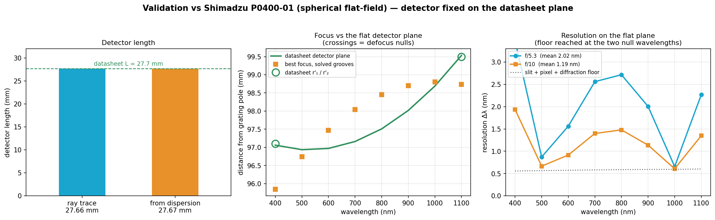
The catch: one chirp, two sharp wavelengths. The C1 needed to cancel defocus is different at every wavelength — 0.59 at 400 nm, 0.13 at 700 nm, 0.33 at 1100 nm. A real grating has one C1, so it cancels defocus at about two wavelengths (near 510 and 1010 nm) and leaves some everywhere else. That is the flat-field compromise every grating like this makes, and it's why the resolution curve is W-shaped.

Predicted performance (modelled end to end: real lens surfaces, slit, reconstructed grating, pixels):

• Resolution: 0.63–0.68 nm at 1000 and 500 nm, 1.43 nm averaged over 400–1100 nm, 2.1 nm at the 400 nm end.
• Light: about 1 % of the fiber's light lands on the pixels (geometric; coatings, grating and detector efficiency not included).
• Size: fiber to slit 87 mm; the whole optical train fits in about 20 × 9 cm.
• Cost of the sourced optics: ₹66,795 (fiber, two lenses, slit), plus the grating and detector.

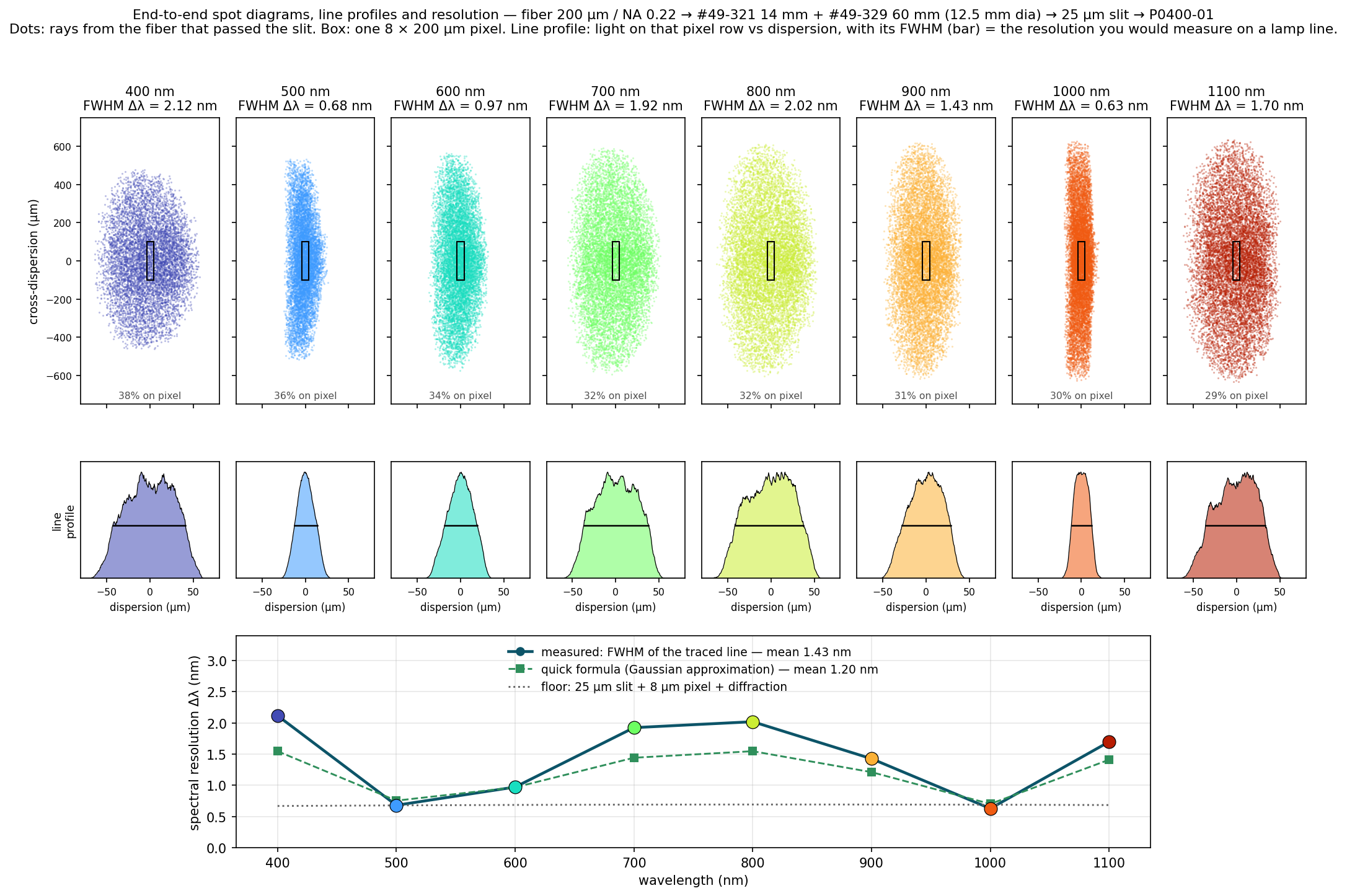
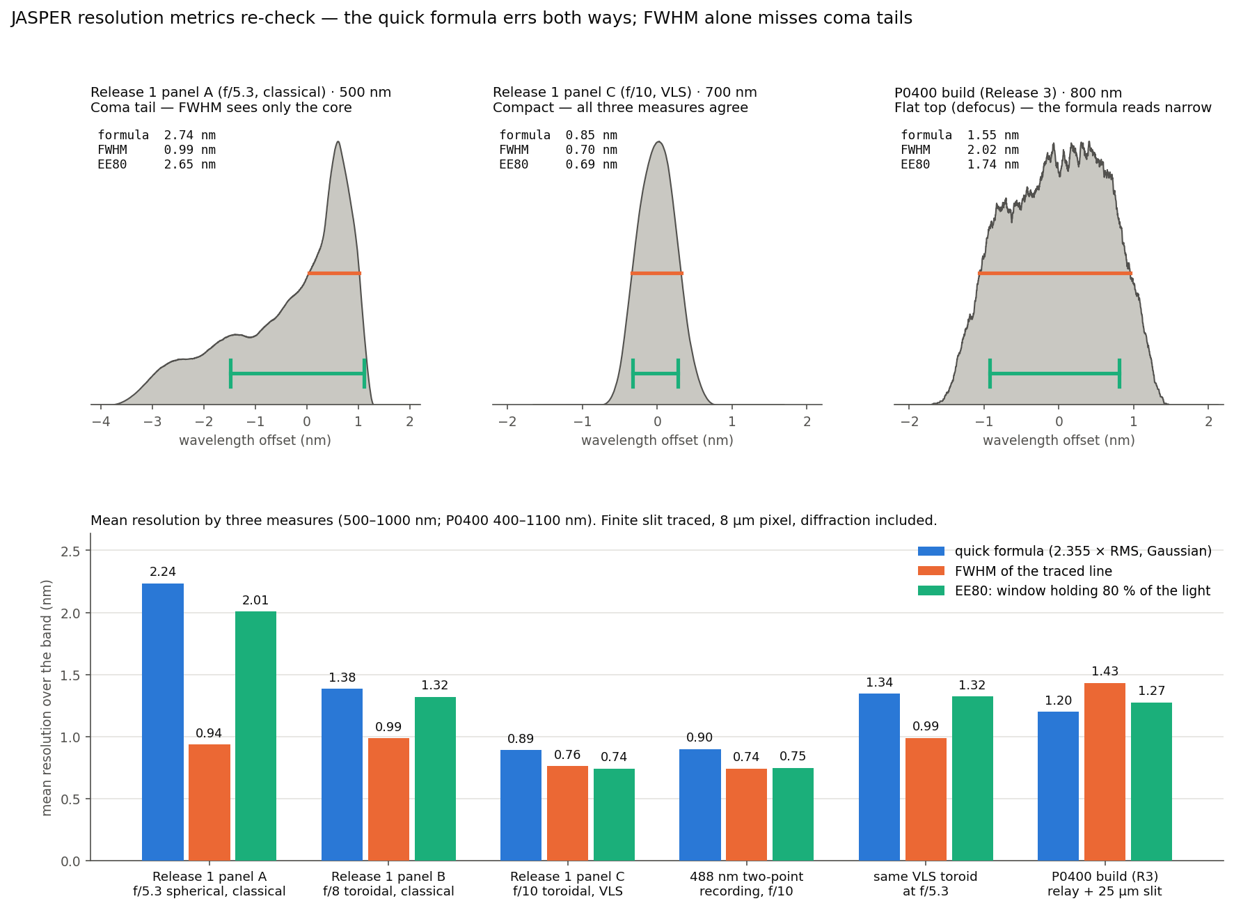
Two corrections to earlier logs. First, how we measure resolution. Earlier logs used a quick formula (2.355 × RMS of the ray spread, with slit, pixel and diffraction added in quadrature), which assumes every line is bell-shaped. We re-checked every headline number against the traced line itself, with the finite slit traced, and now report two widths: the FWHM (what you'd read off a lamp line) and EE80 (the narrowest window holding 80 % of the line's light, which catches tails the FWHM misses). The formula errs both ways. For this P0400 build, defocus makes the lines flat-topped and the formula reads narrow: 1.20 nm vs 1.43 nm FWHM (EE80 1.27 nm). For the Release 1 f/10 design the lines are compact and the formula was conservative: we quoted ~0.9 nm; measured, it is 0.76 nm FWHM / 0.74 nm EE80 (worst 0.93 nm), and a real 488 nm holographic recording of that grating (in the repo) gives 0.74 / 0.75 nm. Without the groove correction, at f/5.3, the line has a sharp core and a long coma tail — 0.94 nm FWHM but 2.0 nm EE80 — so FWHM alone would flatter it. Second, the "0.9 nm at f/5.3" bar in an earlier comparison figure was an idealised bound (defocus cancelled at every wavelength), which no single groove pattern can reach on a flat detector. A real single chirp at f/5.3, detector at best focus, gives ~1.3 nm (EE80; 1.0 nm FWHM). The repo, figure and numbers are updated (resolution_metrics.py).

What's next. Order the parts and a P0400 sample, then measure the grooves directly: scan a thin laser beam across the blank and read the local groove density from the diffraction angle (a 1 l/mm change moves the spot ~0.3 mm at 0.5 m), then check resolution on Hg/Ar lamp lines — it should bottom out near 500 and 1000 nm. The largest remaining loss is vertical: the spherical blank smears each wavelength into a tall line, so only ~30–39 % of the slit light lands on 200 µm pixels; a cylindrical lens in front of the detector should recover most of it.

Code, derivation and parts list (pure NumPy, deterministic): https://github.com/CheckAG/JASPER_VIS_NIR_Optics_Design/tree/main/JASPER_1nm_VLS_simulated  see P0400_VLS_derivation.md and JASPER_P0400_build.md.

Full disclosure: the modelling and code are heavily AI-assisted and human-reviewed; posting it so people who know these gratings can check the assumptions before we buy hardware.