It's been quite a while since I last posted here, so I'll try to make up for that this weekend.

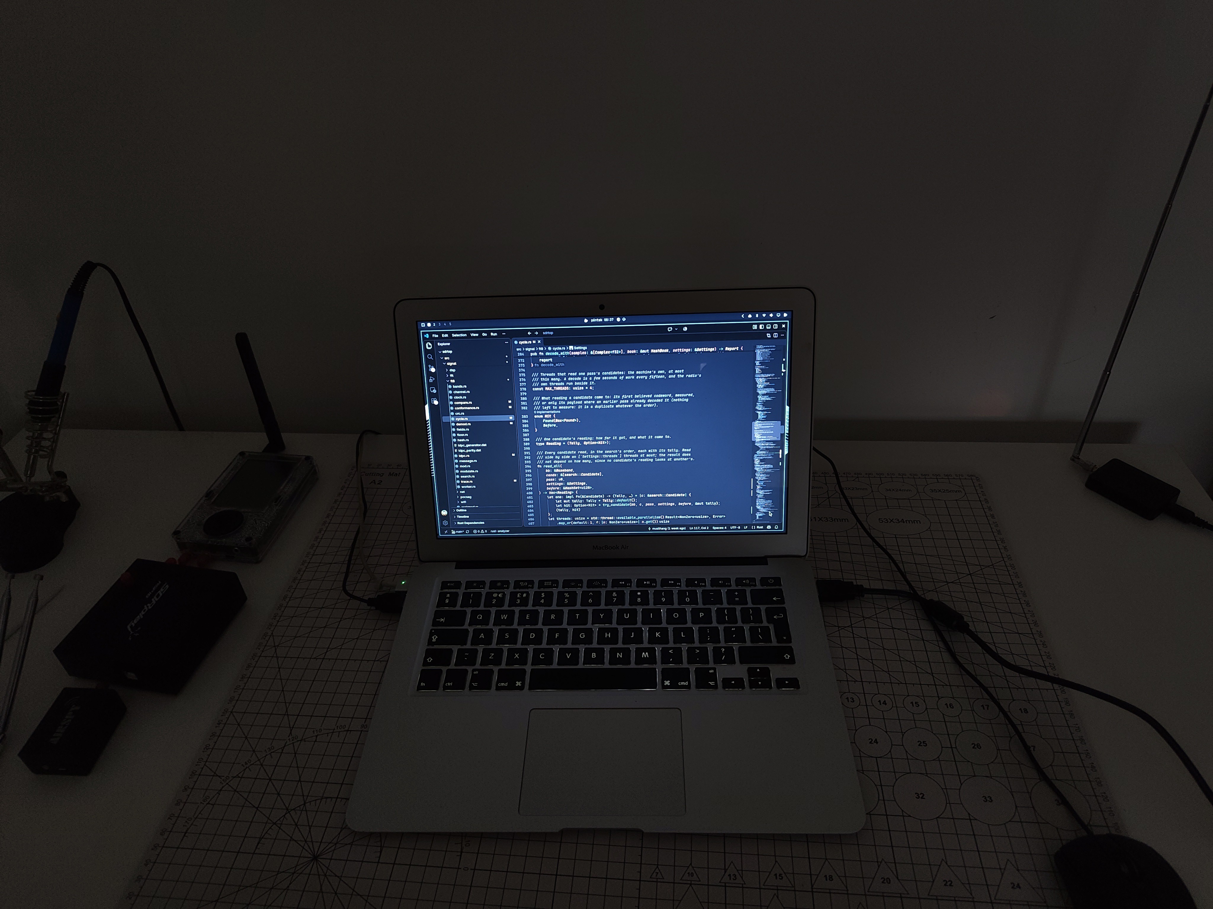
My laptop finally gave up on me, so I'm temporarily switching to my old MacBook Air. Not exactly the upgrade I had in mind, but the work continues.

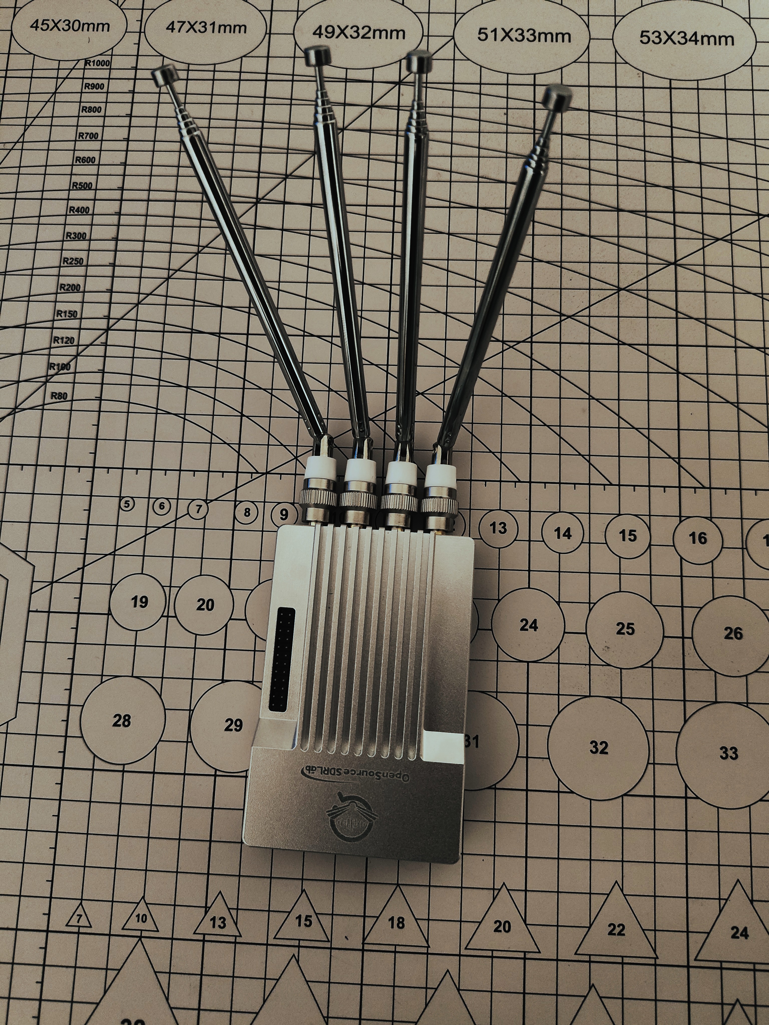
On a brighter note, a new piece of hardware has arrived! The PlutoSky R2 is here, and a huge thank you to OpenSourceSDRLabs for making this possible!

I'm planning to add native support for it in sdrtop. With 56 MHz of bandwidth to play with, I've already got quite a few ideas about what this hardware could be useful for. Still figuring out which directions to explore first.

Plenty of experiments ahead!

Three radios on the desk

October. Time to dive back into the workshop and put hands on the hardware. This year that feels even more true than usual.

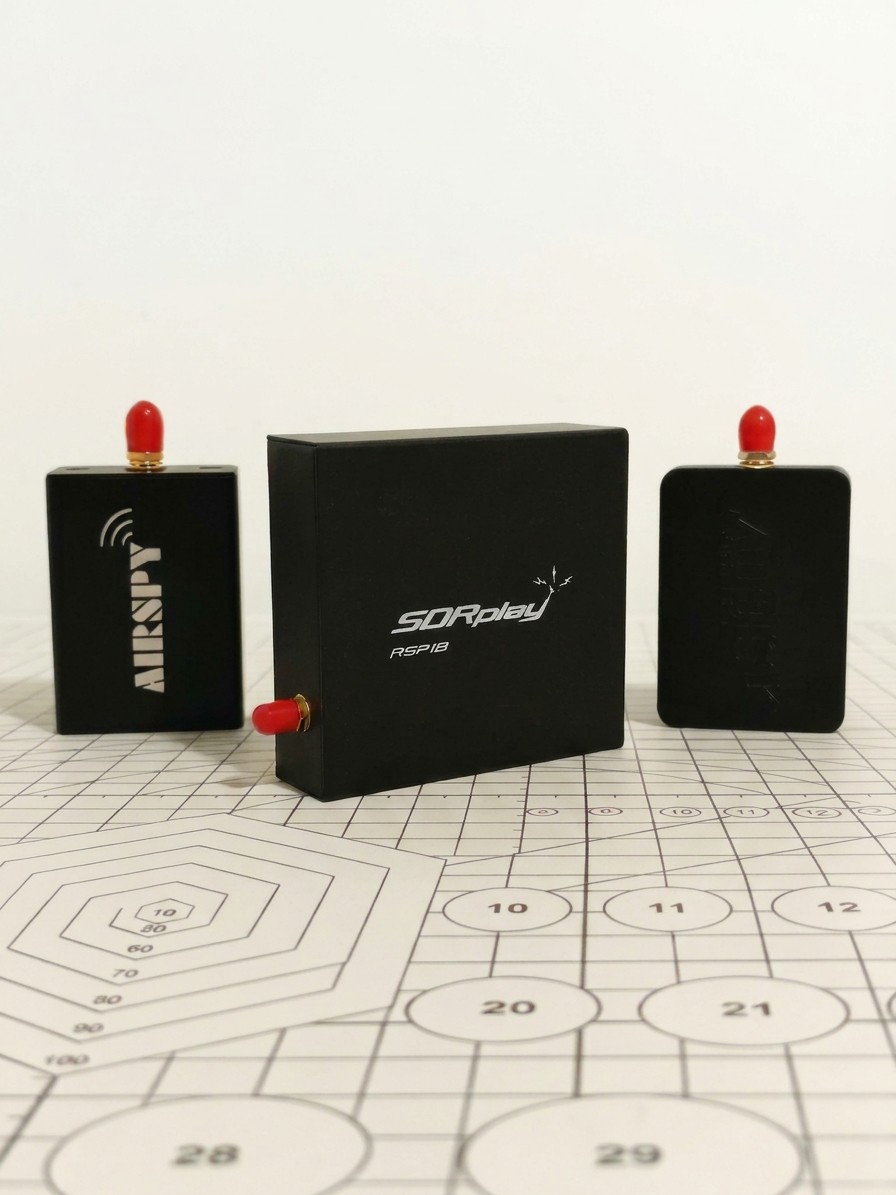
Last few days two packages arrived. SDRplay sent an RSP1B, Airspy sent an HF+ Discovery and an R2. I can't quite believe both said yes. Thanks to both teams. That's not a small thing for a solo project. It is a huge help to the software, me, and anyone who will eventually run sdrtop on these radios.

The immediate next task is obvious. Native support for all three of the above. Same rule as always. Nothing is marked as supported until it has spent some time on this desk, tested for real. Beyond that the door is open. I am not going to list the plans here, but if you've ever looked at a band or signal path and thought 'I could really make something of that with the right front end' then this desk has just gotten a lot more interesting.

And then, in the middle of that, macOS happened.

sdrtop was originally targeted at Linux, and had backends that tried shared libraries the way that Linux does, and the observer mode that reads USB stats from /sys. All perfectly reasonable choices for a desktop app, but completely useless on a Mac... 

And this week almost by accident: macOS. Someone opened an issue from a MacBook with an RTL-SDR. The backends were Linux-only. We chased it down, and proper macOS support is landing. Might even ship this week

Hardware from the vendors. 

A careful bug report from a stranger with a Mac. 

That is how a solo project moves in October.

Whether you're using sdrtop or just want to help me out, even opening an issue can be a great way to contribute.

The latest Wi-Fi work in sdrtop presents two new views: Survey and Frames.

The idea was not to write another application listing nearby networks. There already are too many of those. I was interested to peer one layer deeper into the radio and learn about transmissions on a channel and how they fit with one another in time and what can be derived from a received signal before attempting to decode its payload.

1. Starting with the radio

Wi-Fi is often presented to the user as a collection of network names, signal-strength bars and channel numbers. Those are useful abstractions, but hide much of the behaviour taking place over the air.

At the physical level, a Wi-Fi transmission is a time varying radio signal. Different frame formats use different signalling structures, and the receiver has to identify a transmission, establish timing, estimate frequency offset and recover enough of the PHY information to understand what it is looking at.

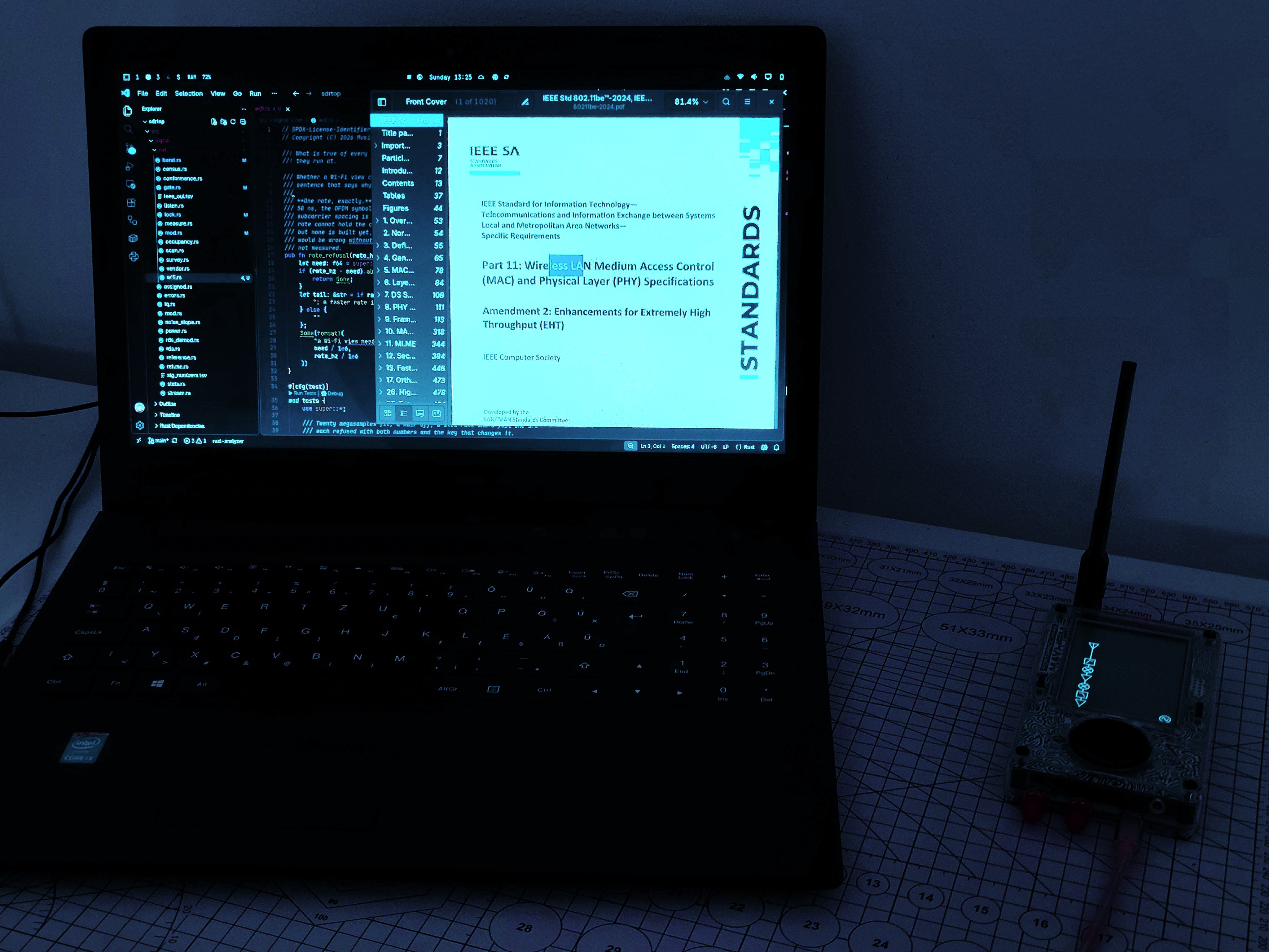
The reference for this work is the IEEE 802.11-2024 standard, with the applicable amendments consulted where necessary. Rather than treating a successful decode as the sole proof of existence of a frame, the receiver is designed to account for detected activity even when the available information is incomplete.

That distinction is important. A frame whose payload cannot be decoded may still occupy airtime. A burst detected from a neighbouring channel may still contribute energy to the capture. Neither should silently disappear from the picture simply because they do not fit the simplest decoding path.

The first implementation focuses on the 2.4 GHz band and a single 20 MHz channel at a time.

The reference hardware used during development is the HackRF One, configured at 20 Msps. HackRF One uses 8-bit I/Q samples, so this is a constrained measurement environment, not an ideal laboratory receiver. The receiver, the sample stream and the available processing time all influence what can be established reliably.

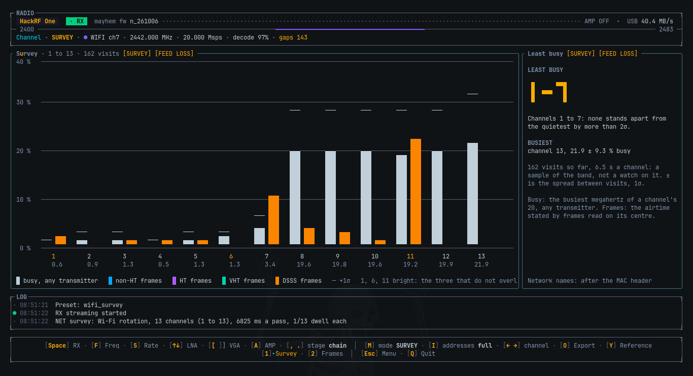
2. Survey: which channel is busy?

First view is Wi-Fi > Channel > Survey.

Its question is deliberately simple: which Wi-Fi channels are busy and which are comparatively quiet?

The survey cycles through the Wi-Fi channel centres, rather than observing them all at once. For the current 2.4 GHz implementation, it means visiting channels 1 through 13 and accumulating observations for each channel.

It is an important detail when interpreting the result: the display is built from measurements accumulated over time, rather than thirteen receivers working in parallel. Each channel is observed during its own sampling interval, the amount of observation time and the coverage achieved is relevant when comparing the results.

The view combines the channel picture with the activity that was detected during those visits, a way to compare the observed busy time, observe where frames have been detected and the relationship between channel positions and their overlapping bandwidths.

Why visit every channel rather than just channels 1, 6 and 11?

Those three are commonly used as a simplified channel planning reference because they are separated, in a many 2.4 GHz deployments. But they aren't only frequencies at which a receiver can encounter Wi-Fi activity, a scan only those centres could miss networks on other channels, even if their energy is present in the wider band.

The Survey therefore visits the individual channel centres, a network is generally most usefully observed with the receiver tuned to its own channel, while energy from overlapping or adjacent ones can influence what the receiver sees.

The intended use is more exploratory rather than prescriptive: a channel that appears quieter during a time of survey isn't necessarily the best channel for every device or every moment. The scan has a finite observation time, traffic varies and interference isn't necessarily Wi-Fi. The measurements describe what the receiver observed during the survey: not a guarantee of future network performance.

That is the difference between displaying a ranking and claiming to have solved channel selection.

3. Frames: from a channel summary to individual transmissions

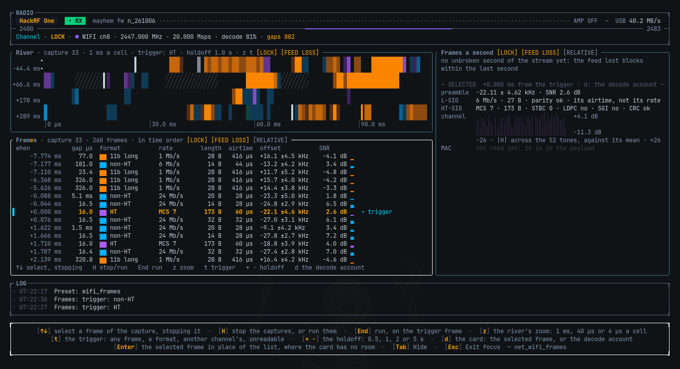
Survey provides the overview. Wi-Fi → Channel → Frames is where the view becomes more specific.

Frames locks the receiver to one channel and presents the detected activity in arrival order. Rather than looking at an accumulated channel statistic only, it becomes possible to look at the sequence of transmissions and the gaps between them.

This changes the questions that are possible to ask.

Is the channel occupied by a few long transmissions or many short ones? How close are the detected bursts to each other? What PHY formats and rates are being observed? How much time does an individual frame occupy?

These are questions about the radio activity rather than the presence of a network.

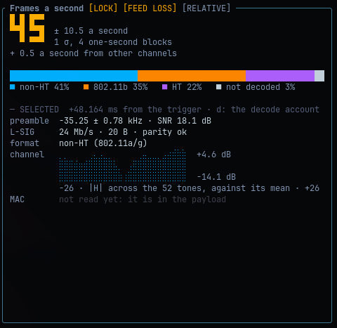
The view records the information the receiver can establish at this stage (timing, detected format, rate and length where recovered, frequency offset, signal-to-noise information and estimated airtime). Selecting a frame provides a closer look at its available measurements.

This is not a promise that every payload is decoded. The current work focuses on identifying and characterising transmissions at the PHY level. A detected frame can still be useful to the analysis when its payload is unavailable or cannot be decoded.

4. Three time scales for the same activity

One of the core choices the team made while working on the design of Frames is that a single time scale isn't enough. The display offers three different views of the timeline.

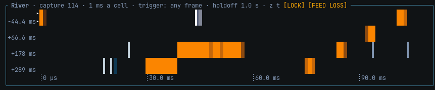
Load: 1 ms per cell

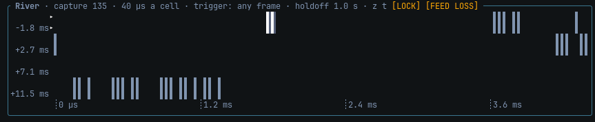
Rhythm: 40 µs per cell

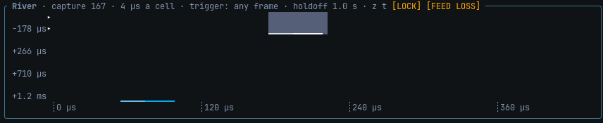
Anatomy: 4 µs per cell

Each has its own purpose.

Load: the larger picture

At 1 ms per cell, the timeline allows us to see the overall pattern better. It makes it easier to see when the channel is busy, which periods have the longest durations, and how transmissions are spread out over a larger period.

This is the perspective we want to start with when the question is about overall traffic structure and not the fine details of one burst.

Rhythm: the gaps between transmissions

At 40 µs per cell, the time line can be used to observe the spacing between transmissions.

Wi-Fi is not a continuous medium of energy. Devices contend for access to it, and the time between frames is part of this contending. At this scale, shorter bursts of activity and the spaces between them become apparent.

The IEEE 802.11 MAC and PHY standards define timing relationships used in the protocol. The relationships give context to a captured sequence, but a visual absence is not evidence of causality in this case.

Anatomy: looking closely at a burst

At 4 µs per cell, the timeline is good for taking a closer look at the structure of the transmission.

At this zoom level, it's possible to see details that get lost when a lot of microseconds get crammed into one cell. It's easier to get a feel for how the apparent length of a burst relates to what the receiver found in its frame.

The three scales aren't three different ways of measuring the same thing. It's three different ways of looking at the same observed timeline, with progressively more information about timing.

It's like looking at an oscilloscope, only you can zoom in and out by adjusting the time base. Zoom out to see the big picture, zoom in to see the details of an event. But either way, you aren't adding any information that wasn't already there in the sample stream.

5. Airtime: how long does a frame occupy the medium?

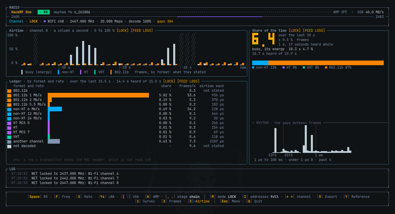
One particularly useful value in frames is airtime.

A PHY data rate alone can't tell you how long a transmission will occupy the channel; the rate tells you how much information is getting through per second under a particular PHY configuration. The actual duration depends on the length of the entire frame and the particular physical-layer structure that is required to transmit it.

For supported frame formats, the receiver uses the decoded PHY information, including rate and length, to calculate the transmission duration. For legacy OFDM frames, the SIGNAL field contains information that lets the receiver calculate the rate and length. The 802.11b path uses its own PLCP header and timing.

The relevant PHY procedures are specified in the IEEE 802.11 standard. The implementation follows the appropriate format instead of trying to treat every burst of radio waves as if it's the same kind of transmission.

Why is this useful?

Think of two frames which were observed on a same channel. One was short: it was transmitted with a modest bitrate. The other was long: it was transmitted on a higher bitrate. Judging by the rate alone, we cannot say how much the two frames differ in their use of the medium. Time on channel (airtime) gives a more direct estimation.

It also adds information to simply observing a point in time. A frame isn't an instantaneous moment in time; it takes some duration to be transmitted. And the duration between frames is equally informative.

There are also practical limits to how much information can be derived from airtime. An observation of airtime can only be made as precise as the amount of information the receiver could correctly recover for any given frame. A frame which cannot be classified, or which does not contain the bits necessary to determine its airtime should not be considered to have an airtime with an unrealistically precise duration. Receiver losses and incomplete observations can also impact the comprehension of a sequence of frames.

6. Why build a receiver instead of only measuring energy?

A spectrum display can indicate the presence of energy, but energy itself does not define the structure of a Wi-Fi transmission.

The Wi-Fi receiver therefore uses the structure defined by the standard as a basis for detecting candidate transmissions and distinguishing a signal that belongs to the tuned channel from activity that could be from an adjacent channel.

For OFDM, the preamble provides the starting point for detection and timing and frequency-offset estimation. The receiver then checks for the expected training structure before treating the burst as a transmission on the selected channel. This is because a signal from a nearby channel can sometimes look like a valid preamble at the initial stages of detection.

The implementation takes care to account for legacy DSSS transmissions used by 802.11b. An OFDM-only perspective would provide an incomplete view of the 2.4 GHz spectrum where legacy frames are present. The standard provides separate signalling structures for these PHY families, therefore different detection paths are needed for each.

The important engineering principle is that the receiver should not mistake a plausible initial detection for a confirmed frame of the expected format.

The relevant reference is the PHY description in IEEE 802.11-2024, including the OFDM and DSSS/HR-DSSS clauses. The IEEE 802.11 working group provides background on the standards family and its revisions.

7. What this version does not claim

This is an early step in a larger Wi-Fi measurement bench. Not a complete Wi-Fi protocol analyser.

The current Survey and Frames views are concerned with channel activity and frame-level observations. They do not yet provide the full set of capabilities needed for a complete network census, detailed per-device accounting or a comprehensive transmitter-conformance test.

A few are particularly important:

• One channel at a time. Frames is locked to one channel. Survey rotates across channel centres, so it cannot observe every channel continuously and simultaneously.

• Finite capture bandwidth. The current HackRF path operates at 20 Msps around a tuned channel centre. Signals and spectral features outside the captured bandwidth cannot be reconstructed from samples that were never received.

• Incomplete decoding is still possible. A burst can be detected without all of its fields being recovered. Measurements should reflect that distinction.

• The receiver has its own limitations. Sample resolution, gain, filtering, frequency reference, noise and dropped samples can affect the result. A measurement of another transmitter is also a measurement made through the receiving instrument.

• Airtime is not throughput. The duration of a frame is not the same as useful application data delivered per second, and a single capture does not reveal the complete state of a network.

These are not reasons to avoid measurement. They are reasons to state clearly what was measured, under which conditions, and with what degree of confidence.

The longer-term direction is to build on these observations with more detailed airtime analysis, network-level information and transmitter measurements. Those are separate steps, each requiring its own validation.

8. Implementation and references

The Wi-Fi receiver is being developed on the sdrtop's existing NET architecture. Where the underlying algorithms are genuinely similar, there's intention to reuse established DSP and measurement infrastructure, while isolating protocol specific behaviour to the relevant standard.

The implementation is in Rust and uses the projects own receiver and measurement paths. It is not intended to be a graphical Wi-Fi dashboard, nor a replacement for every existing network-analysis tool. It is a radio bench that just happens to run in a terminal.

References:

• sdrtop source code
• sdrtop v0.6.8 release notes
• IEEE Std 802.11-2024
• IEEE 802.11 Working Group
• IEEE Std 802.11be-2024, Extremely High Throughput amendment
• HackRF One documentation

The standard defines the protocol. The receiver implementation turns a subset of that definition into measurements to obtain. The interface is where the measurements are made actionable by a person inspecting them.

That is the direction I want sdrtop to head towards: less black-box interpretation and more visibility on actual evidence with a clear distinction between what the radio observed and what one could reasonably assume based on that evidence.

Bluetooth may take a break for a moment, while I look into Wi-Fi.

This weekend was spent reading standard and updating the plan so that the first version cannot be accused of lying: a cheap SDR on one 20 MHz channel cannot do what a lab box can.

What I want to be displayed on screen, in order:

• What is this channel up to? Every single burst, including the ones we cannot fully decode, and for how long does it occupy the air?
• Who is here? Later, when there are addresses.
• Is that transmitter any good? Clock offset, signal quality, compared to the limits in the standard's own specification.
• What does the path look like? How much is it echoing the room, in nanoseconds and metre.

The first pass at this requires only step 1: detecting the burst, reading the short header that contains rate and length information, and counting how long in the air it was. 

                    IQ @ 20 Msps
                         │
                         ▼
              ┌─────────────────────┐
              │  burst detector     │
              │  (short training)   │
              └──────────┬──────────┘
                         │
            ┌────────────┼────────────┐
            ▼            ▼            ▼
         this         neighbour      noise
        channel       channel
            │            │
            ▼            ▼
     read rate &      count energy
     length from      as adjacent
     the header       airtime
            │
            ▼
     ┌──────────────┐
     │  airtime     │
     │  by rate &   │
     │  format      │
     └──────────────┘

A full decoding of the payload is not needed in the first pass; frames that we cannot read still consume medium capacity, and that must be shown or the utilisation number is fiction.

This is how the wifi menu will look like:

Wi-Fi
  Channel     1 Survey   2 Frames   3 Airtime   ← first release
  Room        1 Paths    2 Motion
  Network     1 Census
  Transmitter 1 Bench

Menu gets its own Wi-Fi heading (Survey / Frames / Airtime first). Code is moving.

Edit:

while reading the IEEE 802.11 docs I happened upon a test vector which used the first 72 characters of Schiller's Ode to Joy as the payload. 😂

Including the typo in "Fire-insired"

So here I am, reading Wi-Fi documentation, and I stumble across poetry encoded in a Rust byte array.

Here's what that looks like in Rust:

/// The example's PSDU (Annex I.1, Table I-1): a MAC header, the first 72
/// characters of Schiller's "Ode to Joy" with LF line breaks (the typo in
/// "Fire-insired" is the annex's own, and deliberate), and the FCS.
#[rustfmt::skip]
pub const MESSAGE: [u8; 100] = [
    0x04, 0x02, 0x00, 0x2E, 0x00, 0x60, 0x08, 0xCD, 0x37, 0xA6,
    0x00, 0x20, 0xD6, 0x01, 0x3C, 0xF1, 0x00, 0x60, 0x08, 0xAD,
    0x3B, 0xAF, 0x00, 0x00, b'J', b'o', b'y', b',', b' ', b'b',
    b'r', b'i', b'g', b'h', b't', b' ', b's', b'p', b'a', b'r',
    b'k', b' ', b'o', b'f', b' ', b'd', b'i', b'v', b'i', b'n',
    b'i', b't', b'y', b',', b'\n', b'D', b'a', b'u', b'g', b'h',
    b't', b'e', b'r', b' ', b'o', b'f', b' ', b'E', b'l', b'y',
    b's', b'i', b'u', b'm', b',', b'\n', b'F', b'i', b'r', b'e',
    b'-', b'i', b'n', b's', b'i', b'r', b'e', b'd', b' ', b'w',
    b'e', b' ', b't', b'r', b'e', b'a', 0x67, 0x33, 0x21, 0xB6,
];

Thanks for reading.

In ham radio, a QSL card says one thing: “I heard you, thanks for the contact.” This is one of those, logged.

Two signals received

sdrtop got written up on the RTL-SDR Blog and on the Adafruit blog. Both posts picked out exactly the parts I care about: no audio on purpose, numbers that go [STALE] when RX stops, and a signal path written from scratch. Which means somebody read the README all the way down. Thank you both, and hello to everyone who came over from there.

One package incoming

sdrtop has a rule: a radio gets native support only after it has physically sat on my desk. It’s a good rule. It’s also why the README has a row of grey badges that mean “should work, but nobody has told me yet”.

So I reached out to Airspy. I showed them my project. They said yes, and an Airspy R2 and an HF+ Discovery engineering sample are already on their way. I’m very grateful to them for their support.

The plan when they land:

• a native backend for each device
• tested on real hardware, not from a datasheet
• documented in the docs: how the backend works, what was measured, and any limitations found
• the badge turns green once verified

Until then, the grey stays grey. That’s the rule.

So, funny story. For about a month, sdrtop had a Bluetooth Low Energy receiver that decoded every packet perfectly. Every packet I made, that is. Point it at an actual phone and the CRC failed. Every packet, every device, every single time. Meanwhile the test suite was green from top to bottom, smiling at me.

A receiver that works on everything you make and nothing anyone else makes is a very specific kind of broken. This is the story of finding out which kind, with the code, the dead ends, and the moment I realised the bug had been introducing itself by name for weeks.

Quick map: what a BLE packet looks like on air

Keep this picture in your head, it's the whole plot:

  ┌──────────┬────────────────┬────────┬─────────────┬──────────┐
  │ preamble │ access address │ header │   payload   │  CRC-24  │
  │  8 bits  │    32 bits     │16 bits │ 0-37 bytes  │ 24 bits  │
  └──────────┴────────────────┴────────┴─────────────┴──────────┘
  │◄──── NOT whitened ───────►│◄──────── whitened (scrambled) ──►│
          known in advance            depends on channel number

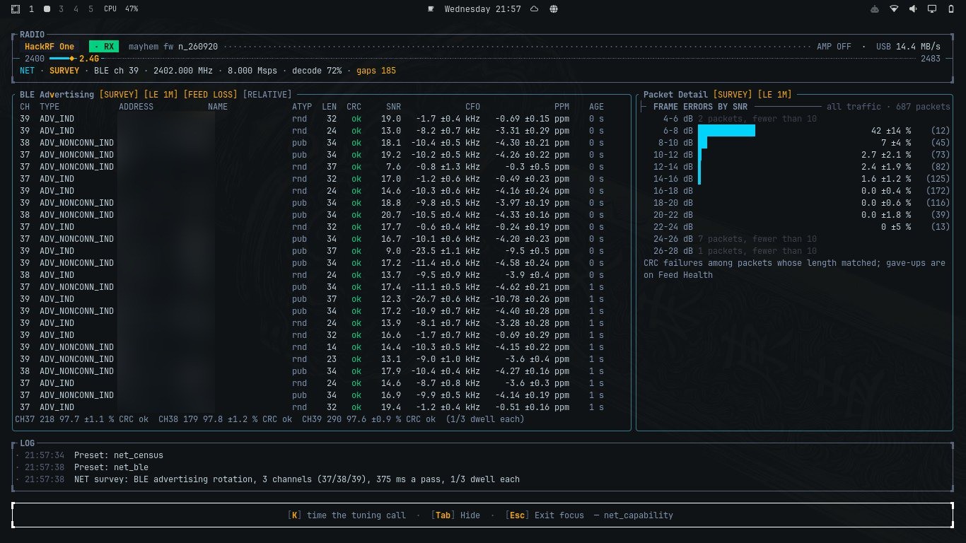
The first 40 bits are known: on the advertising channels the access address is always 0x8E89BED6. Everything after that is scrambled ("whitened") by a 7-bit shift register seeded from the channel number, then checked by a 24-bit CRC.

The suspects (all guilty of something, none of this)

The cruel part: every theory I had pointed at a real bug. I fixed each one, things got better, and the CRC kept failing like it hadn't noticed.

theory                      real bug?   fixed?   CRC passes?
──────────────────────────  ─────────   ──────   ───────────
sub-symbol timing phase     yes         yes      no
CRC byte order              "yes"*      "yes"*   no
carrier frequency offset    measured    ruled    out
no anti-alias filter        yes         yes      no
interpolation bias          yes         partly   no
ADC overload (phone on      yes!        yes      no
the antenna, max gain)
low per-bit SNR             measured    ruled out

* hold that thought

 A couple of these deserve a closer look, because the numbers were genuinely fun.

The overload one. Phone pressed against the antenna, AMP on, LNA and VGA maxed. The survey panel read a peak of +0.6 dBFS and a noise floor of -9.1 dBFS. That's not a receiver, that's a microphone held inside a drum. Backing the gain off gave -10.1 dBFS peak, a -48.6 dBFS floor, and for the first time ever a sane modulation reading on real air. Real fix. CRC: still failing.

The SNR one. Maybe the bits were just noise? So I measured against ground truth: slide a 40-bit window over each capture and count how many bits differ from the known preamble plus access address. As a control, I ran the same search over pure random bits, 200 times:

ground-truth check: wrong bits out of 40 (best window)

pure noise, 200 trials   ███████████████  never better than 7
real captures            ██               0 to 5   ← that's a real signal

The bits were coming through clean. And then the clue that, in hindsight, solved the case:

preamble + access address        header           payload ...
  ✔ ✔ ✔ ✔ ✔ ✔ ✔ ✔ ✔ ✔ ✔ ✔ ✔ ✔ ✔ ✔ │ ✘ ✘ ✘ ✘ ✘ ✘ ✘ ✘ ✘ ✘ ✘ ✘
                                  ▲
                 clean up to exactly here, garbage after,
                 the SAME garbage, every time, both ways I computed it

Look at that boundary. Now look at the packet map above. I didn't. I wrote it down, nodded wisely, and walked off in completely the wrong direction.

"It's not a bug, it's my flat"

I dumped raw IQ to disk and averaged the amplitude in 16-sample blocks across the one capture that matched cleanly:

amplitude (block average) across one capture

 1.1 │          ████
 0.8 │         ██████
 0.4 │█████████        
 0.2 │                 ████████████████████████████
     └────────────────────────────────────────────── samples
      0       512  696                          1409
               ◄──►
         ~46 symbols of signal, then nothing

 Conclusion at the time: the bursts here are only ~46 symbols long, enough for a preamble and access address and nothing else. Bad antenna, bad flat, no bug. I marked the task closed.

Then I looked around.

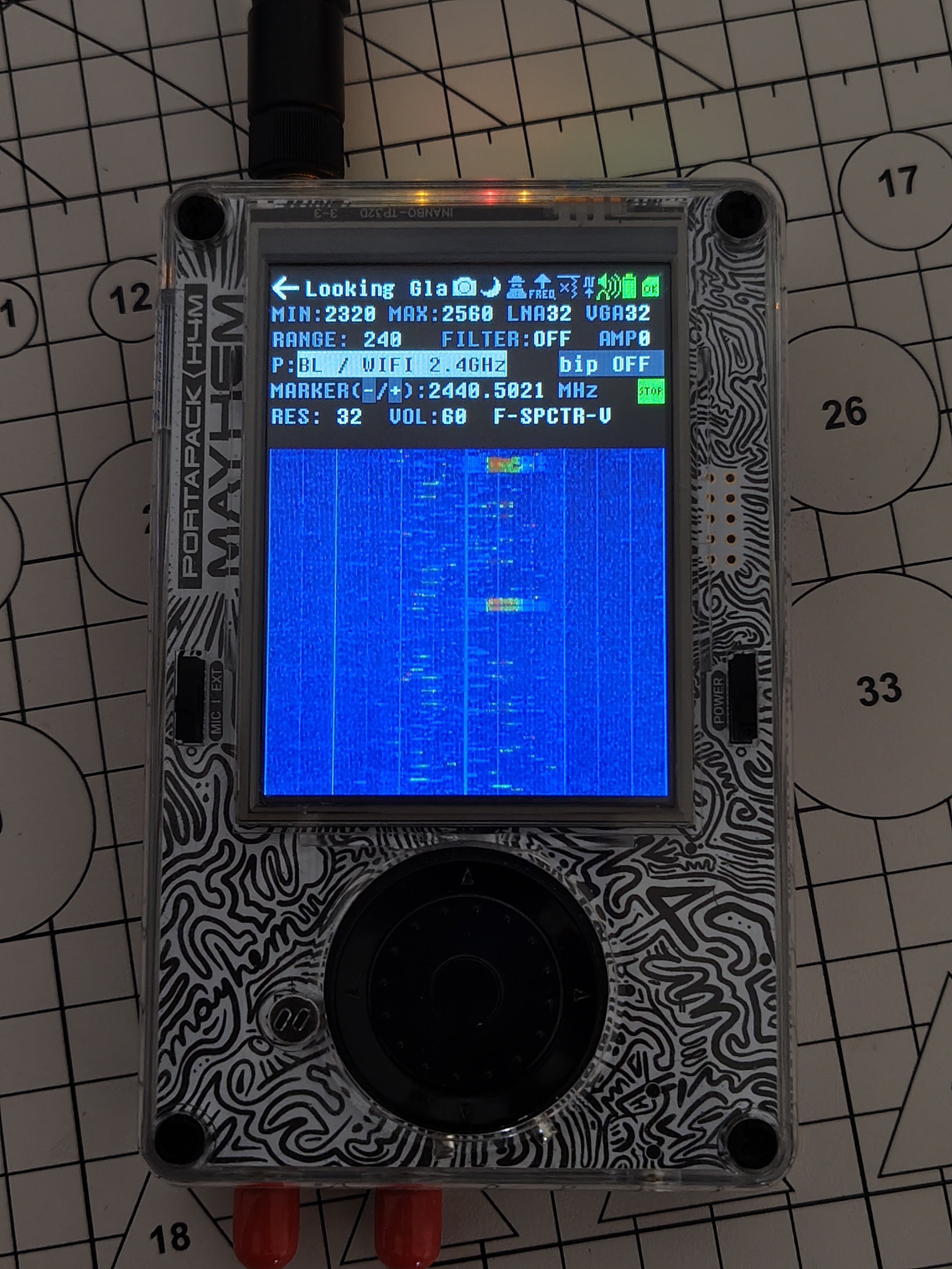
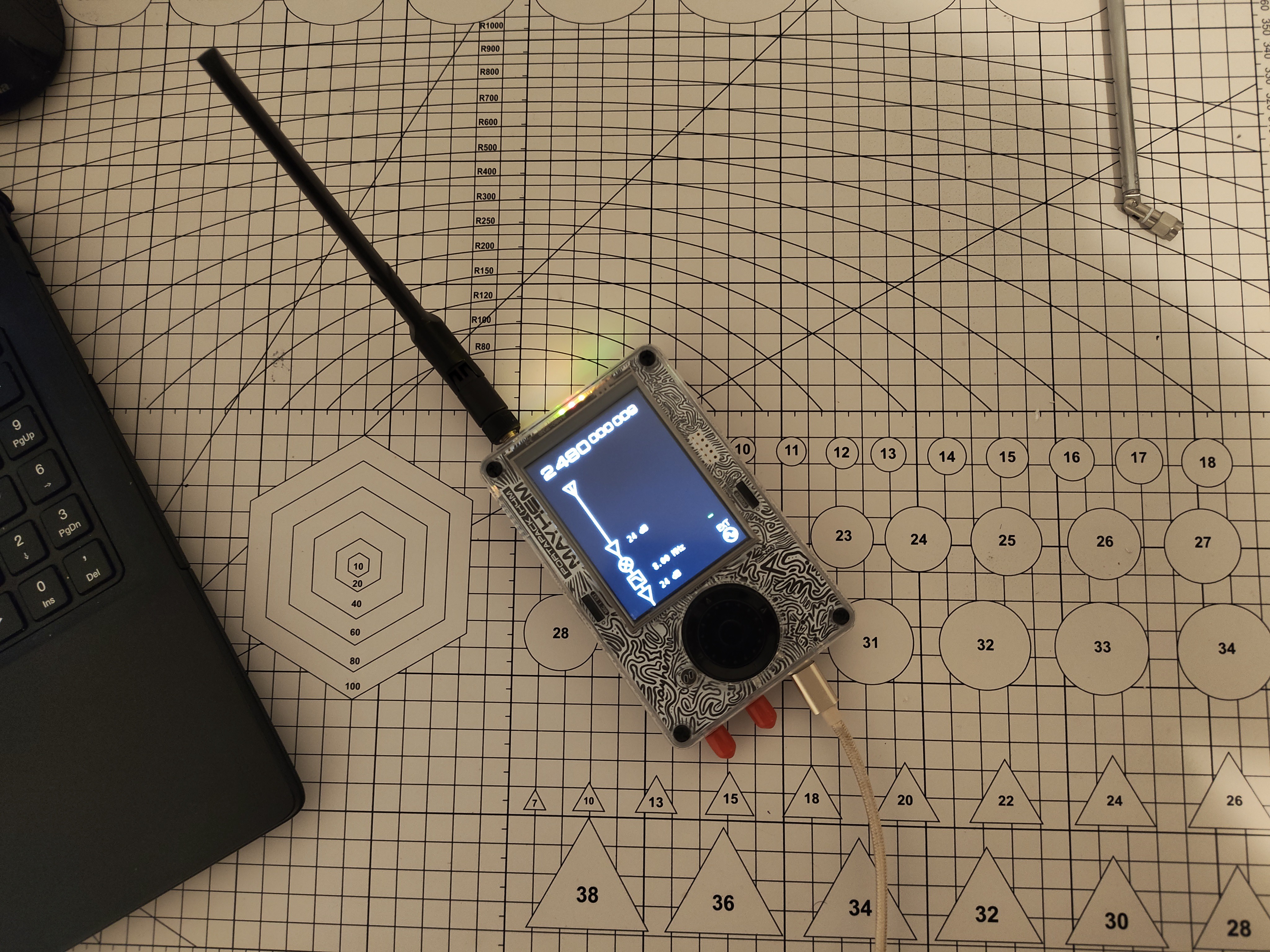
The lab. Population: one HackRF, one antenna, and about ten BLE devices I can hear through the walls.

I live in a three-storey panel block. My phone lists eight to ten Bluetooth devices at any moment: my phones, the TV, the neighbours' phones and watches. A building full of advertisers does not produce nothing but 46-symbol slivers. My theory was clever. The building was louder. Case reopened.

A second red herring: decode 840%

The same afternoon I added a decode-load readout to the NET header. First reading, HackRF at 20 Msps: decode 840%. Of real time. One 131 072-sample block took about 36 ms to process, for 6.6 ms of signal. That's not a receiver, that's a very slow archive.

It also exposed that dropped blocks were being spliced together as if continuous, which produces exactly "clean sync word, then garbage". New favourite theory! Then arithmetic killed it: at 4 Msps a block is 32.8 ms and a packet is at most 0.4 ms, so only a percent or two of packets can straddle a gap. Splicing can spoil some packets. Not every single one.

The experiment that ended it: take the app out of the loop

The question I'd somehow never asked cleanly: is it the live pipeline, or the receiver itself? So I cut the app out completely and recorded eight seconds of lossless IQ on advertising channel 37:

hackrf_transfer -r ch37_8msps.iq -f 2402000000 -s 8000000 \
                -l 32 -g 24 -a 0 -n 64000000

 Then a four-step isolation, each step cutting the suspect list in half:

                ┌──────────────────────────┐
                │  8 s lossless recording  │
                └────────────┬─────────────┘
                 ┌───────────┴────────────┐
                 ▼                        ▼
      ┌────────────────────┐   ┌──────────────────────────┐
      │ sdrtop receiver,   │   │ independent Python RX,   │
      │ offline            │   │ zero shared code,        │
      │                    │   │ everything from the spec │
      └─────────┬──────────┘   └────────────┬─────────────┘
                ▼                           ▼
        20 packets, 0 CRC          12 packets, 10 CRC ✔
        → not the pipeline         → recording is fine,
                                     reference is right
                                            │
                     reference's good air bits
                                            ▼
                      ┌───────────────────────────────┐
                      │ sdrtop's whiten() + decode()  │
                      └───────────────┬───────────────┘
                                      ▼
                              0 of 8 pass  → it's in HERE

A false CRC pass is a one-in-16-million fluke, so ten passes means: the recording is fine, the Python is right, and I am wrong. One afternoon. After a month. 

The design choice that mattered: the Python receiver had to be independent. If I'd ported my own whitening into it to save time, it would have reproduced the bug and happily confirmed it.

Culprit #1: the right sequence at the wrong moment

BLE whitens with a 7-bit LFSR, polynomial:

The spec draws it as a Galois register. I'd built a Fibonacci one. Simplified, here's the difference:

Hackaday's code block doesn't support Rust :(

// What I had: Fibonacci. Feedback from positions 2 and 6 into 0.
fn step_fibonacci(r: &mut [bool; 7]) -> bool {
    let out = r[6];
    let fb = r[2] ^ r[6];
    for i in (1..7).rev() { r[i] = r[i - 1]; }
    r[0] = fb;
    out
}

// What the spec draws: Galois. Position 6 out and back into 0,
// XORed into position 4 on the way.
fn step_galois(r: &mut [bool; 7]) -> bool {
    let out = r[6];
    for i in (1..7).rev() { r[i] = r[i - 1]; }
    r[0] = out;
    r[4] ^= out;
    out
}

 Now the fun part: I didn't pick Fibonacci by accident, I tested my way into it. I brute-forced every tap pair on a 7-bit register and found four that give a maximal-length sequence. Maximal length alone doesn't say which polynomial you have, so I added a second check: the output must obey the recurrence the polynomial implies.

#[test]
fn the_output_satisfies_its_own_recurrence() {
    // x^7 + x^4 + 1  ⇒  o[t] = o[t-3] xor o[t-7]
    let o = whitening_sequence(37, 300);
    for t in 7..o.len() {
        assert_eq!(o[t], o[t - 3] ^ o[t - 7]);
    }
}

 Both tests are correct. Both pass for both register types. A Galois and a Fibonacci register with the same polynomial generate the same sequence, but from the same starting contents they start at different points in it:

spec's seed → Galois:    0 1 1 0 1 0 0 1 1 1 0 1 ...  ✔
spec's seed → Fibonacci: 0 1 1 0 1 1 1 0 0 1 0 ...   ✘
                         └──┬──┘ └─────┬─────────
                     agree for a few   then never again

 (The bit patterns above are illustrative, not the real sequences. The shape is the point.) My tests pinned down the polynomial. Nothing ever tested the structure.

Culprit #2: the comment that lied

Remember the asterisk? Early on I'd "fixed" the CRC byte order, with a comment saying a real transmitter had confirmed it. Real hardware had never passed a single CRC. The comment was a belief wearing a lab coat.

I compute the CRC in its reflected form (standard, and correct: it matches the RevEng catalogue's check value, 0xC25A56 for "123456789"). In that form the first bit on air is the lowest one, so the lowest byte arrives first:

// before: read like a big-endian number ("confirmed on hardware")
let crc = (b[0] as u32) << 16 | (b[1] as u32) << 8 | b[2] as u32;

// after: reflected CRC, lowest octet first on air
let crc = b[0] as u32 | (b[1] as u32) << 8 | (b[2] as u32) << 16;

Fixing them one at a time, the reference's 8 good packets through my decoder:

before any fix          0 / 8   garbage types, garbage lengths
+ Galois LFSR           0 / 8   types and lengths RIGHT, CRC still ✘
+ CRC octet order       8 / 8   ✔✔✔✔✔✔✔✔

Why the tests were green the whole time

This is the part I actually want you to take away

  test transmitter                     receiver
  ┌──────────────┐                    ┌──────────────┐
  │ encode()     │                    │ decode()     │
  │   whiten() ──┼── same function ───┼── whiten()   │
  │   crc order ─┼── same convention ─┼── crc order  │
  └──────┬───────┘                    └──────▲───────┘
         └──── GFSK → noise → filter → slice ┘

  wrong on both sides, in the same way  →  test passes ✔

Every round-trip test checked that my code agreed with itself. It always did. Perfectly consistent, never correct. And the "clean up to one exact bit" clue? That bit is exactly where the whitening starts. Deterministic garbage, because the whitening depends only on the channel. Plausible header fields, because the two registers agree for the first few bits. A failing CRC, because it sits at the end, long after they diverge. Every clue was measured correctly and read as a property of the signal. They were properties of the code.

The fix, and the tests that guard it

Two real over-the-air packets from that recording, a SCAN_RSP and an ADV_NONCONN_IND, both verified by the independent reference, are now permanent tests:

#[test]
fn a_real_over_the_air_packet_dewhitens_to_a_clean_crc() {
    // Air bits captured on channel 37, CRC verified by an
    // independent receiver that shares no code with this crate.
    let mut bits = REAL_SCAN_RSP_AIR_BITS.to_vec();
    whiten(&mut bits, 37);
    let pkt = pdu::decode(&bits).expect("a packet");
    assert!(pkt.crc_ok);
}

#[test]
fn a_second_real_packet_of_another_type_also_passes() { /* ... */ }

 They're the first tests in the project built from bits my own code didn't produce, which is exactly why they're the first ones that could have caught this. Same recording, before: 0 of 20. After: 7 of 19. My first real CRC-clean Bluetooth packets, from real devices in my building. I may have made a noise.

Bonus round 1: from 1% to real time

Correct, but slow. Same two seconds of recorded traffic, and every step had to keep every CRC pass:

time to process 2 s of signal                       CRC passes

start                 ████████████████████   208 s       16
decode per byte,
not per sample        █                     10.1 s       17
shared discriminator  ▊                     8.9 s       17
shared phase search   ▍                     4.1 s       17
FFT matched filter    ▏                     1.2 s       17   ~170× faster

 My favourite find: the old matched filter did a modulo per tap per sample. At 4 Msps that's 570 million divisions a second. Sometimes optimisation is just "stop doing the silly thing". Live in the app afterwards: decode 72% while surveying all three advertising channels.

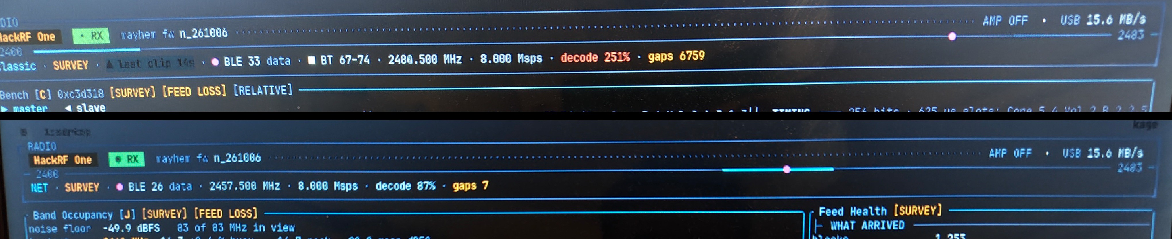
Today, two views side by side. The NET survey runs at 87%. The Classic view, with eight classic Bluetooth receivers running on top of BLE, still sits at 251% with the gaps piling up. That one’s next on the list.

(Also: my first benchmark timed one cold block including FFT planning and allocations, and overstated the cost twofold. I nearly threw away a good change because of it. Warm up, then average.)

Bonus round 2: it only heard neighbours who agreed with my crystal

Fixed CRC, real time, done? The Python reference still heard about twice as much: 17 against 33. Nine of the missing packets came from one device, heard once in twelve transmissions.

The matched filter correlates phase coherently across the 40-µs sync word. A crystal 15 kHz off rotates the phase by 0.6 of a cycle over that window, and the correlation falls apart:

coherence at the trigger, the "missing" device

no correction      ▓▓▓▓▓▓▓▓░░░░░░░░░░░░  0.26-0.39   threshold 0.387
corrected 10-15k   ▓▓▓▓▓▓▓▓▓▓▓▓▓▓▓▓▓░░░  0.70-0.91

So the receiver wasn't listening to the building. It was listening to the part of the building whose crystals happened to agree with my HackRF's. In a standard that allows ±150 ppm, which is ±360 kHz.

The fix: correlate the frequency track instead of the phase. A carrier offset is just a constant added to the frequency track, and Pearson's correlation removes constants by construction:

 phase domain (old)              frequency domain (new)
  offset = rotation               offset = constant shift
  ⟳ breaks coherence              ⇧ Pearson ignores it
       ✘                               ✔  whole ±360 kHz

And the threshold isn't picked, it's measured. Under pure noise the statistic is roughly normal with variance 1/N_eff, so N_eff was measured through the receiver's own front end (107.8 for LE 1M), the tail checked out to 4.5 sigma, and the threshold set at 6 sigma, ≈ 0.58: about one false trigger per billion samples. A test re-measures it, so if I ever change the front end, the threshold fails loudly instead of quietly changing meaning.

Result: 28 CRC-clean packets against the reference's 33, up from 17. The missing device decodes 12 out of 12. Live, it even caught one sitting 120 kHz off.

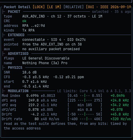
And this is what a packet looks like now: CRC clean, every figure read the way the Bluetooth test suite defines it, each with its ± and its limit. Not bad for a receiver that once only understood itself.

The lesson, now baked into how I build things

The real fix wasn't two functions, it was a habit. When I later wrote the decoder for BLE connection packets, the encoder and decoder were again written together, so I knew they'd agree with each other whatever I did. So that test suite has one test holding the decoder to the Bluetooth Core spec's own published sample packets, bytes I didn't make:

#[test]
fn the_cores_own_sample_pdus_read_as_labelled() {
    // Encryption sample data from the Core specification itself:
    // LL_ENC_REQ, LL_START_ENC_REQ, ... decoded as the spec labels them.
}

And the measurement side now has a whole reference transmitter in closed form (an erf-based GFSK model, exact to f64) that shares zero code with the receive chain. Same rule, bigger hammer.

Still open, because sdrtop doesn't do fake happy endings: five packets still trigger and then fail to decode, and the live load runs higher than offline for reasons I haven't measured yet. Suspects exist. Answers don't. Yet.

TL;DR

• If your transmitter and receiver share code, your round-trip test is just your code high-fiving itself. Test against bits you didn't make.
• Separate the layers before you start theorising. One lossless recording beat twenty live sessions.
• "Confirmed on real hardware" in a comment is a claim. Where's the measurement?
• The strangest clue is usually the most precise one.
• When the room disagrees with your theory, believe the room.

The receiver never had a reception problem. It was a perfect listener who only understood one speaker in the world: itself. Now it understands the neighbours too. Mostly. Sorry, neighbours.