David Prutchi
-
Added new videos of DOLPi and DOLPi-MECH operating in in real time
09/21/2015 at 15:30 • 0 commentsDOLPi-MECH operating in real-time:
DOLPi operating in real-time (full analysis mode):
DOLPi operating in polarization-difference mode:
-
Added 5-minute video describing DOLPi project
09/20/2015 at 23:24 • 0 commentsSemifinals video added to YouTube and linked to Hackaday.io.
-
Released new version of DOLPi whitepaper
09/19/2015 at 20:39 • 0 comments![]()
The latest and greatest version of the DOLPi whitepaper is now available for download in pdf format at: http://www.diyphysics.com/wp-content/uploads/2015/09/DOLPi_Polarimetric_Camera_D_Prutchi_2015_v2.pdf
This 80-page paper presents the development and construction of two low-cost polarimetric cameras based on the Raspberry Pi 2.“DOLPi-MECH” is a filter-wheel-type camera capable of performing full Stokes analysis, while the electro-optic based “DOLPi” camera performs full linear polarimetric analysis at higher frame rate. Complete Python code for polarimetric imaging is presented. Various applications for the cameras are described, especially its use for locating mines and unexploded ordinance in humanitarian demining operations.
-
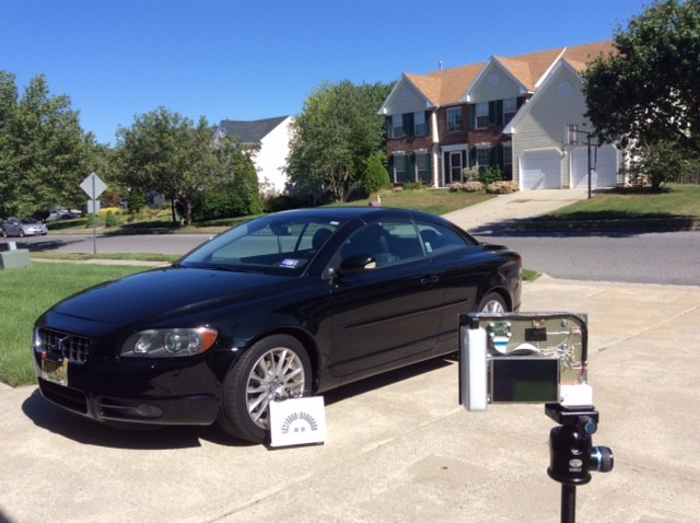
Added two outdoor videos demonstrating DOLPi and DOLPi-Mech
09/14/2015 at 15:41 • 0 commentsAdded two YouTube videos demonstrating the operation of DOLPi and DOLPi-Mech in real-time. The polarimetric cameras are imaging my daughter's car parked in the driveway. A linear polarization fan target by the front wheel provides a reference for the color scale:
This is the scene viewed in normal color vision:
![]()
This is the DOLPi-MECH real-time video:
This is the DOLPi real-time video:
-
Videos of DOLPi and DOLPi-MECH imaging target in real-time
09/14/2015 at 15:31 • 0 commentsAdded two demonstration operation videos to YouTube - One of DOLPi and one of DOLPi-MECH imaging a test target in real-time:
-
Real-Time HSV Representation of Polarization Working
09/09/2015 at 23:46 • 2 commentsA popular way of presenting polarization information is by recognizing that the three main polarization components – polarization intensity, Degree of Linear Polarization, and Angle of Polarization - are analogous to the color components of brightness, saturation, and hue. The HSV (Hue, Saturation, Value) model provides better contrast and more quantifiable information about a scene’s polarization than the simple RGB merge that I have been using so far. Here are the "normal" and RGB polarization images for my test target:
![]()
![]()
In contrast, the HSV representation really hones in on polarized light:
![]()
WOW!!!! Everything that is not linearly polarized just went completely dark, while polarized light on the other hand really pops out!!! Can you spot the LCDs on my calculator and digital calipers? Also notice the perfect encoding of linear angle of polarization (AoP) by color.
It's remarkable that there is no back-illumination involved whatsoever. The three images above were acquired by DOLPi-MECH under identical conditions on my workbench. Illumination comes solely from overhead fluorescent lights and some late-afternoon sunlight seeping through the window blinds.
The Python code to render the HSV image is:
    #convert images to signed double (int16)
    image0_d=np.int16(image0)
    image90_d=np.int16(image90)
    image45_d=np.int16(image45)
    image135_d=np.int16(image135)
    imageLHCP_d=np.int16(imageLHCP)
    imageRHCP_d=np.int16(imageRHCP)
    #calculate Stokes parameters
    stokesI=image0_d+image90_d+1
    stokesQ=image0_d-image90_d
    stokesU=image45_d-image135_d
    stokesV=imageLHCP_d-imageRHCP_d
    #calculate polarization parameters
    polInt=np.sqrt(1+np.square(stokesQ)+np.square(stokesU))  #Linear Polarization Intensity
    polDoLP=polInt/stokesI   #Degree of Linear Polarization
    polAoP=0.5*(np.arctan2(stokesU,stokesQ))  #Angle of Polarization
    polDoCP=(2*np.absolute(stokesV))/polInt  #Degree of Circular Polarization

    #prepare DOLPi HSV image
    H=np.uint8((polAoP+(3.1416/2))*(180/3.1416))
    S=np.uint8(255*(polDoLP/np.amax(polDoLP)))
    V=np.uint8(255*(polInt/np.amax(polInt)))

    imageDOLPiHSV=cv2.merge([H,S,V])
    DOLPiHSVinBGR=cv2.cvtColor(imageDOLPiHSV,cv2.COLOR_HSV2BGR)
    cv2.imshow("DOLPi_HSV",DOLPiHSVinBGR)
You may notice that OpenCV (cv2) assumes the following ranges for the HSV parameters:
Hue = H = 0 to 180 (please refer to the main project's white paper for an explanation)
Saturation = S = 0 to 255
Value (Intensity) = V = 0 to 255
The HSV tuple is then converted into a BGR tuple that can be displayed through cv2.imshow (cv2 uses BGR instead of RGB encoding for color images).
Next - I'll work on integrating the polarization analysis and real-time HSV into the electro-optic DOLPi's code and compare its performance against that of the much slower but more precise DOLPI-MECH.
Here is the complete code as it currently stands for DOLPi-MECH:
# DOLPiMech2.py # # This Python program demonstrates the DOLPi_Mech polarimetric camera. # # A servo motor rotates a polarization filter wheel in front of the # Raspberry Pi camera. An Adafruit PWM Servo HAT drives the servo. # # (c) 2015 David Prutchi, Ph.D., licensed under MIT license # (MIT, opensource.org/licenses/MIT) # # #import the necessary packages from picamera.array import PiRGBArray from picamera import PiCamera import time import cv2 from Adafruit_PWM_Servo_Driver import PWM import numpy as np import matplotlib.pyplot as plt def dispStokes(stokesI, stokesQ, stokesU, stokesV): #Function dispStokes - Save and optionally display Stokes parameters plt.figure("Stokes") plt.subplot(2,2,1) plt.imshow(stokesI) plt.axis('off') plt.title("Stokes I") # plt.subplot(2,2,2) plt.imshow(stokesQ) plt.axis('off') plt.title("Stokes Q") # plt.subplot(2,2,3) plt.imshow(stokesU) plt.axis('off') plt.title("Stokes U") # plt.subplot(2,2,4) plt.imshow(stokesV) plt.axis('off') plt.title("Stokes V") # plt.savefig('Stokes.png',bbox_inches='tight') plt.show(block=False) def dispPol(polInt, polDoLP, polAoP, polDoCP): #Function dispPol - Save and optionally display polarization parameters plt.figure("pol") plt.subplot(2,2,1) plt.imshow(polInt) plt.axis('off') plt.title("Linear Pol Intensity") # plt.subplot(2,2,2) plt.imshow(polDoLP) plt.axis('off') plt.title("DoLP") # plt.subplot(2,2,3) plt.imshow(polAoP) plt.axis('off') plt.title("AoP") # plt.subplot(2,2,4) plt.imshow(polDoCP) plt.axis('off') plt.title("DoCP") # plt.savefig('polarization.png',bbox_inches='tight') plt.show(block=False) # Initialise the Adafruit PWM HAT using the default address pwm = PWM(0x40) pwm.setPWMFreq(60) # Set PWM frequency to 60 Hz servoMin = 180 # Min pulse length out of 4096 servoMax = 615 # Max pulse length out of 4096 # Servo PWM values for different filter wheel positions servoNone = 615 # PWM setting for open window servo0=541 # PWM setting for 0 degree filter servo90=468 # PWM setting for 90 degree filter servo45=395 # PWM setting for 45 degree filter servo135=321 # PWM setting for -45 degree (=135 degree) filter servoLHCP=247 # PWM setting for LHCP filter servoRHCP=180 # PWM setting for RHCP filter #Raspberry Pi Camera Initialization #---------------------------------- #Initialize the camera and grab a reference to the raw camera capture camera = PiCamera() camera.resolution = (320, 240) #camera.resolution = (640, 480) #camera.resolution = (1280,720) camera.framerate=30 rawCapture = PiRGBArray(camera) camera.led=False #Auto-Exposure Lock #------------------ # Wait for the automatic gain control to settle time.sleep(2) # Now fix the values camera.shutter_speed = camera.exposure_speed camera.exposure_mode = 'off' gain = camera.awb_gains camera.awb_mode = 'off' camera.awb_gains = gain #Initialize flags loop=True #Initial state of loop flag first=False #Flag to skip display during first loop video=False #Use video port? Video is faster, but image quality is significantly #lower than using still-image capture while loop: #grab an image from the camera with no filter pwm.setPWM(0, 0, servoNone) time.sleep(0.5) rawCapture.truncate(0) camera.capture(rawCapture, format="bgr",use_video_port=video) imageNone=rawCapture.array #grab an image from the camera with linear polarizer at 0 degrees pwm.setPWM(0, 0, servo0) time.sleep(0.1) #Wait for filter wheel to move rawCapture.truncate(0) camera.capture(rawCapture, format="bgr",use_video_port=video) image0=cv2.cvtColor(rawCapture.array,cv2.COLOR_BGR2GRAY) #grab an image from the camera with linear polarizer at 90 degrees pwm.setPWM(0, 0, servo90) time.sleep(0.1) rawCapture.truncate(0) camera.capture(rawCapture, format="bgr",use_video_port=video) image90=cv2.cvtColor(rawCapture.array,cv2.COLOR_BGR2GRAY) #grab an image from the camera with linear polarizer at 45 degrees pwm.setPWM(0, 0, servo45) time.sleep(0.1) rawCapture.truncate(0) camera.capture(rawCapture, format="bgr",use_video_port=video) image45=cv2.cvtColor(rawCapture.array,cv2.COLOR_BGR2GRAY) #grab an image from the camera with linear polarizer at -45 degrees (=135 degrees) pwm.setPWM(0, 0, servo135) time.sleep(0.1) rawCapture.truncate(0) camera.capture(rawCapture, format="bgr",use_video_port=video) image135=cv2.cvtColor(rawCapture.array,cv2.COLOR_BGR2GRAY) #grab an image from the camera with LHCP filter pwm.setPWM(0, 0, servoLHCP) time.sleep(0.1) rawCapture.truncate(0) camera.capture(rawCapture, format="bgr",use_video_port=video) imageLHCP=cv2.cvtColor(rawCapture.array,cv2.COLOR_BGR2GRAY) #grab an image from the camera with RHCP filter pwm.setPWM(0, 0, servoRHCP) time.sleep(0.1) rawCapture.truncate(0) camera.capture(rawCapture, format="bgr",use_video_port=video) imageRHCP=cv2.cvtColor(rawCapture.array,cv2.COLOR_BGR2GRAY) #convert images to signed double (int16) image0_d=np.int16(image0) image90_d=np.int16(image90) image45_d=np.int16(image45) image135_d=np.int16(image135) imageLHCP_d=np.int16(imageLHCP) imageRHCP_d=np.int16(imageRHCP) #calculate Stokes parameters stokesI=image0_d+image90_d+1 stokesQ=image0_d-image90_d stokesU=image45_d-image135_d stokesV=imageLHCP_d-imageRHCP_d #calculate polarization parameters polInt=np.sqrt(1+np.square(stokesQ)+np.square(stokesU)) #Linear Polarization Intensity polDoLP=polInt/stokesI #Degree of Linear Polarization polAoP=0.5*(np.arctan2(stokesU,stokesQ)) #Angle of Polarization polDoCP=(2*np.absolute(stokesV))/polInt #Degree of Circular Polarization #prepare DOLPi HSV image H=np.uint8((polAoP+(3.1416/2))*(180/3.1416)) S=np.uint8(255*(polDoLP/np.amax(polDoLP))) V=np.uint8(255*(polInt/np.amax(polInt))) #The following block is just for debugging #----------------------------------------- #plt.imshow(H) #plt.axis('off') #plt.title("H=AoP") #plt.colorbar() #plt.show() # #plt.imshow(S) #plt.axis('off') #plt.title("S=polDoLP") #plt.colorbar() #plt.show() # #plt.imshow(V) #plt.axis('off') #plt.title("V=polInt") #plt.colorbar() #plt.show() #prepare DOLPi RGB image R=image0 B=image90 G=image45 imageDOLPi=cv2.merge([B,G,R]) cv2.imshow("Image_DOLPi",imageDOLPi) #Display DOLPi preview image imageDOLPiHSV=cv2.merge([H,S,V]) DOLPiHSVinBGR=cv2.cvtColor(imageDOLPiHSV,cv2.COLOR_HSV2BGR) cv2.imshow("DOLPi_HSV",DOLPiHSVinBGR) #cv2.imshow("Image_DOLPi",cv2.resize(imageDOLPi,(320,240),interpolation=cv2.INTER_AREA)) #Display DOLP image k = cv2.waitKey(1) #Check keyboard for input if k == ord('x'): # wait for x key to exit loop=False # Save and Prepare to leave # ------------------------- # pwm.setPWM(0, 0, servoNone) #return filter wheel to no-filter position #display and save calculated polarization parameters dispStokes(stokesI, stokesQ, stokesU, stokesV) dispPol(polInt, polDoLP, polAoP, polDoCP) #save images cv2.imwrite("imageNone.jpg",imageNone) cv2.imwrite("image0.jpg",image0) cv2.imwrite("image90.jpg",image90) cv2.imwrite("image45.jpg",image45) cv2.imwrite("image135.jpg",image135) cv2.imwrite("imageLHCP.jpg",imageLHCP) cv2.imwrite("imageRHCP.jpg",imageRHCP) cv2.imwrite("RGBpol.jpg",cv2.merge([B,G,R])) cv2.imwrite("HSVpol.jpg",DOLPiHSVinBGR) #exit time.sleep(10) cv2.destroyAllWindows() quit -
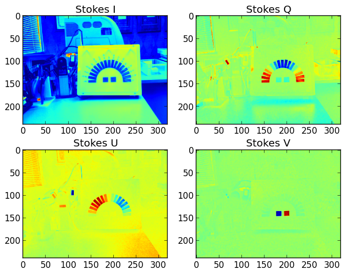
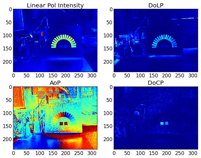
Complete Stokes Analysis Code for DOLPi-Mech
09/09/2015 at 20:11 • 1 commentI completed the code for complete Stokes polarization analysis for DOLPi-MECH.
I have the camera aimed at my linear polarizer fan target. The two squares on the middle bottom are circular polarizers. This is how the scene looks without polarization-capable vision:
![]()
This is the linear RGB polarization encoding (my default real-time preview):
![]()
These are the complete Stokes parameters. Note that the last parameter (V) relates to circular polarization, correctly identifying the two circular polarizers and their handedness:
![]()
This is the polarization analysis:
![]()
By coincidence, the penholder where I put my digital calipers was standing by the target, and the LCDs show brightly in the LPI image.
Finally, this is the Python code:
# DOLPiMechComplete.py # # This Python program demonstrates the DOLPi_Mech polarimetric camera. # # A servo motor rotates a polarization filter wheel in front of the # Raspberry Pi camera. An Adafruit PWM Servo HAT drives the servo. # # (c) 2015 David Prutchi, Ph.D., licensed under MIT license # (MIT, opensource.org/licenses/MIT) # # #import the necessary packages from picamera.array import PiRGBArray from picamera import PiCamera import time import cv2 from Adafruit_PWM_Servo_Driver import PWM import numpy as np import matplotlib.pyplot as plt def dispStokes(stokesI, stokesQ, stokesU, stokesV): #Function dispStokes - Save and optionally display Stokes parameters plt.figure("Stokes") plt.subplot(2,2,1) plt.imshow(stokesI) plt.title("Stokes I") # plt.subplot(2,2,2) plt.imshow(stokesQ) plt.title("Stokes Q") # plt.subplot(2,2,3) plt.imshow(stokesU) plt.title("Stokes U") # plt.subplot(2,2,4) plt.imshow(stokesV) plt.title("Stokes V") # plt.savefig('Stokes.png',bbox_inches='tight') plt.show(block=False) def dispPol(polInt, polDoLP, polAoP, polDoCP): #Function dispPol - Save and optionally display polarization parameters plt.figure("pol") plt.subplot(2,2,1) plt.imshow(polInt) plt.title("Linear Pol Intensity") # plt.subplot(2,2,2) plt.imshow(polDoLP) plt.title("DoLP") # plt.subplot(2,2,3) plt.imshow(polAoP) plt.title("AoP") # plt.subplot(2,2,4) plt.imshow(polDoCP) plt.title("DoCP") # plt.savefig('polarization.png',bbox_inches='tight') plt.show(block=False) # Initialise the Adafruit PWM HAT using the default address pwm = PWM(0x40) pwm.setPWMFreq(60) # Set PWM frequency to 60 Hz servoMin = 180 # Min pulse length out of 4096 servoMax = 615 # Max pulse length out of 4096 # Servo PWM values for different filter wheel positions servoNone = 615 # PWM setting for open window servo0=541 # PWM setting for 0 degree filter servo90=468 # PWM setting for 90 degree filter servo45=395 # PWM setting for 45 degree filter servo135=321 # PWM setting for -45 degree (=135 degree) filter servoLHCP=247 # PWM setting for LHCP filter servoRHCP=180 # PWM setting for RHCP filter #Raspberry Pi Camera Initialization #---------------------------------- #Initialize the camera and grab a reference to the raw camera capture camera = PiCamera() camera.resolution = (320, 240) #camera.resolution = (640, 480) #camera.resolution = (1280,720) camera.framerate=30 rawCapture = PiRGBArray(camera) camera.led=False #Auto-Exposure Lock #------------------ # Wait for the automatic gain control to settle time.sleep(2) # Now fix the values camera.shutter_speed = camera.exposure_speed camera.exposure_mode = 'off' gain = camera.awb_gains camera.awb_mode = 'off' camera.awb_gains = gain #Initialize flags loop=True #Initial state of loop flag first=False #Flag to skip display during first loop video=False #Use video port? Video is faster, but image quality is significantly #lower than using still-image capture while loop: #grab an image from the camera with no filter pwm.setPWM(0, 0, servoNone) time.sleep(0.5) rawCapture.truncate(0) camera.capture(rawCapture, format="bgr",use_video_port=video) imageNone=rawCapture.array #grab an image from the camera with linear polarizer at 0 degrees pwm.setPWM(0, 0, servo0) time.sleep(0.1) #Wait for filter wheel to moves rawCapture.truncate(0) camera.capture(rawCapture, format="bgr",use_video_port=video) image0=cv2.cvtColor(rawCapture.array,cv2.COLOR_BGR2GRAY) #grab an image from the camera with linear polarizer at 90 degrees pwm.setPWM(0, 0, servo90) time.sleep(0.1) rawCapture.truncate(0) camera.capture(rawCapture, format="bgr",use_video_port=video) image90=cv2.cvtColor(rawCapture.array,cv2.COLOR_BGR2GRAY) #grab an image from the camera with linear polarizer at 45 degrees pwm.setPWM(0, 0, servo45) time.sleep(0.1) rawCapture.truncate(0) camera.capture(rawCapture, format="bgr",use_video_port=video) image45=cv2.cvtColor(rawCapture.array,cv2.COLOR_BGR2GRAY) #grab an image from the camera with linear polarizer at -45 degrees (=135 degrees) pwm.setPWM(0, 0, servo135) time.sleep(0.1) rawCapture.truncate(0) camera.capture(rawCapture, format="bgr",use_video_port=video) image135=cv2.cvtColor(rawCapture.array,cv2.COLOR_BGR2GRAY) #grab an image from the camera with LHCP filter pwm.setPWM(0, 0, servoLHCP) time.sleep(0.1) rawCapture.truncate(0) camera.capture(rawCapture, format="bgr",use_video_port=video) imageLHCP=cv2.cvtColor(rawCapture.array,cv2.COLOR_BGR2GRAY) #grab an image from the camera with RHCP filter pwm.setPWM(0, 0, servoRHCP) time.sleep(0.1) rawCapture.truncate(0) camera.capture(rawCapture, format="bgr",use_video_port=video) imageRHCP=cv2.cvtColor(rawCapture.array,cv2.COLOR_BGR2GRAY) #convert images to signed double (int16) image0_d=np.int16(image0) image90_d=np.int16(image90) image45_d=np.int16(image45) image135_d=np.int16(image135) imageLHCP_d=np.int16(imageLHCP) imageRHCP_d=np.int16(imageRHCP) #calculate Stokes parameters stokesI=image0_d+image90_d stokesQ=image0_d-image90_d stokesU=image45_d-image135_d stokesV=imageLHCP_d-imageRHCP_d #calculate polarization parameters polInt=np.sqrt(1+np.square(stokesQ)+np.square(stokesU)) #Linear Polarization Intensity polDoLP=polInt/stokesI #Degree of Linear Polarization polAoP=0.5*(np.arctan2(stokesU,stokesQ)) #Angle of Polarization polDoCP=(2*np.absolute(stokesV))/polInt #Degree of Circular Polarization #prepare DOLPi RGB image R=image0 B=image90 G=image45 imageDOLPi=cv2.merge([B,G,R]) cv2.imshow("Image_DOLPi",imageDOLPi) #Display DOLPi preview image #cv2.imshow("Image_DOLPi",cv2.resize(imageDOLPi,(320,240),interpolation=cv2.INTER_AREA)) #Display DOLP image k = cv2.waitKey(1) #Check keyboard for input if k == ord('x'): # wait for x key to exit loop=False # Save and Prepare to leave # ------------------------- # pwm.setPWM(0, 0, servoNone) #return filter wheel to no-filter position #display and save calculated polarization parameters dispStokes(stokesI, stokesQ, stokesU, stokesV) dispPol(polInt, polDoLP, polAoP, polDoCP) #save images cv2.imwrite("imageNone.jpg",imageNone) cv2.imwrite("image0.jpg",image0) cv2.imwrite("image90.jpg",image90) cv2.imwrite("image45.jpg",image45) cv2.imwrite("image135.jpg",image135) cv2.imwrite("imageLHCP.jpg",imageLHCP) cv2.imwrite("imageRHCP.jpg",imageRHCP) cv2.imwrite("RGBpol.jpg",cv2.merge([B,G,R])) #exit time.sleep(10) cv2.destroyAllWindows() quit -
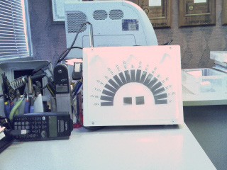
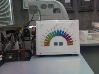
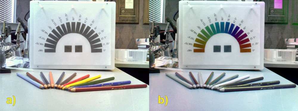
Sample Image Obtained with DOLPi-Mech + Python Code
08/24/2015 at 20:06 • 0 comments![]()
This (picture at right) is a sample image obtained through DOLPi-Mech (linear analysis only, using pictures acquired with analyzer set at 0, 90, and 45 degrees).
The picture on the left is unfiltered (RasPi camera looking through open slot in filter wheel), while the picture on the right is produced by assigning the 0 degree grayscale image to the Red channel, the 90 degree grayscale to Blue, and the 45 degree grayscale to Green.
The sample target is made of polarizing film set at the angles shown. The two bottom squares are circular polarizers. (one LHCP and the other RHCP). We can't tell the difference between the polarizer films because our vision is not sensitive to polarization (to any practical degree), and neither is the RasPi's camera sensor.
Please note that colors in the picture of the right have nothing to do with the actual color of the object, but instead encode the Angle of Polarization. Pure gray tones in the polarimetric image mean that light is unpolarized. Some of the coloring pencils and other stuff in the background shows in color because they partially polarize reflected light as a function of their material, texture, and angle of reflection.
Here is the Python code for the simplest DOLPi-Mech (mechanical filter-wheel, not LCP-based) polarimetric camera:
# DOLPiMech.py
#
# This Python program demonstrates the DOLPi_Mech polarimetric camera.
#
# A servo motor rotates a polarization filter wheel in front of the
# Raspberry Pi camera. An Adafruit PWM Servo HAT drives the servo.
#
# (c) 2015 David Prutchi, Ph.D., licensed under MIT license
# (MIT, opensource.org/licenses/MIT)
#
#
#import the necessary packages
from picamera.array import PiRGBArray
from picamera import PiCamera
import time
import cv2
from Adafruit_PWM_Servo_Driver import PWM
import numpy as np# Initialise the Adafruit PWM HAT using the default address
pwm = PWM(0x40)
pwm.setPWMFreq(60) # Set PWM frequency to 60 Hz
servoMin = 150 # Min pulse length out of 4096
servoMax = 615 # Max pulse length out of 4096
servoNone = 615 # PWM setting for open window
servo0=540 # PWM setting for 0 degree filter
servo90=465 # PWM setting for 90 degree filter
servo45=390 # PWM setting for 45 degree filter# PWM setting function
def setServoPulse(channel, pulse):
pulseLength = 1000000 # 1,000,000 us per second
pulseLength /= 60 # 60 Hz
print "%d us per period" % pulseLength
pulseLength /= 4096 # 12 bits of resolution
print "%d us per bit" % pulseLength
pulse *= 1000
pulse /= pulseLength
pwm.setPWM(channel, 0, pulse)# Rotate filter wheel back and forth to check all is OK
pwm.setPWM(0, 0, servoMin)
time.sleep(1)
pwm.setPWM(0, 0, servoMax)
time.sleep(1)#Raspberry Pi Camera Initialization
#----------------------------------
#Initialize the camera and grab a reference to the raw camera capture
camera = PiCamera()
camera.resolution = (640, 480)
#camera.resolution = (1280,720)
camera.framerate=30
rawCapture = PiRGBArray(camera)
camera.led=False#Auto-Exposure Lock
#------------------
# Wait for the automatic gain control to settle
time.sleep(2)
# Now fix the values
camera.shutter_speed = camera.exposure_speed
camera.exposure_mode = 'off'
gain = camera.awb_gains
camera.awb_mode = 'off'
camera.awb_gains = gain#Initialize flags
loop=True #Initial state of loop flag
first=True #Flag to skip display during first loop
video=False #Use video port? Video is faster, but image quality is significantly
#lower than using still-image capturewhile loop:
#grab an image from the camera at 0 degrees
pwm.setPWM(0, 0, servo0)
time.sleep(0.1) #Wait for filter wheel to moves
rawCapture.truncate(0)
camera.capture(rawCapture, format="bgr",use_video_port=video)
image0 = rawCapture.array
# Select one of the two methods of color to grayscale conversion:
# Blue channel gives better polarization information because wavelengt
# range is limited
# True grayscale conversion gives better gray balance for non-polarized light
#R=image0[:,:,1] #Use blue channel
R=cv2.cvtColor(image0,cv2.COLOR_BGR2GRAY) #True grayscale conversion#grab an image from the camera at 90 degrees
pwm.setPWM(0, 0, servo90)
time.sleep(0.1)
rawCapture.truncate(0)
camera.capture(rawCapture, format="bgr",use_video_port=video)
image90 = rawCapture.array
# Select one of the two methods of color to grayscale conversion:
# Blue channel gives better polarization information because wavelengt
# range is limited
# True grayscale conversion gives better gray balance for non-polarized light
#B=image90[:,:,1] #Use blue channel
B=cv2.cvtColor(image90,cv2.COLOR_BGR2GRAY) #True grayscale conversion#grab an image from the camera at 45 degrees
pwm.setPWM(0, 0, servo45)
time.sleep(0.1)
rawCapture.truncate(0)
camera.capture(rawCapture, format="bgr",use_video_port=video)
image45 = rawCapture.array
# Select one of the two methods of color to grayscale conversion:
# Blue channel gives better polarization information because wavelengt
# range is limited
# True grayscale conversion gives better gray balance for non-polarized light
#G=image45[:,:,1] #Use blue channel
G=cv2.cvtColor(image45,cv2.COLOR_BGR2GRAY) #True grayscale conversionimageDOLPi=cv2.merge([B,G,R])
cv2.imshow("Image_DOLPi",imageDOLPi) #Display DOLP image
#cv2.imshow("Image_DOLPi",cv2.resize(imageDOLPi,(320,240),interpolation=cv2.INTER_AREA)) #Display DOLP image
k = cv2.waitKey(1) #Check keyboard for input
if k == ord('x'): # wait for x key to exit
loop=False# Prepare to leave
# ----------------
#
# Take a "normal" picture
pwm.setPWM(0, 0, servoNone)
time.sleep(0.2)
rawCapture.truncate(0)
camera.capture(rawCapture, format="bgr",use_video_port=video)
imagenone = rawCapture.array
cv2.imwrite("imagenone.jpg",imagenone)
cv2.imwrite("image0.jpg",image0)
cv2.imwrite("image90.jpg",image90)
cv2.imwrite("image45.jpg",image45)
cv2.imwrite("RGBpol.jpg",cv2.merge([B,G,R]))
cv2.imwrite("image0g.jpg",R)
cv2.imwrite("image90g.jpg",G)
cv2.imwrite("image45g.jpg",B)
cv2.destroyAllWindows()
quit -
DOLPi is a Hack-a-Day 2015 Semifinalist!
08/24/2015 at 16:23 • 0 comments"From: no-reply-projects@hackaday.com
Sent: Monday, August 24, 2015 9:39 AM
To: david@...
Subject: Your Project is a Semifinalist in the 2015 Hackaday Prize!
Dear David Prutchi,
Congratulations! We think your DOLPi - RasPi Polarization Camera is awesome and you are one of our top 100 picks for the Hackaday Prize. You are advancing to the next round.
What happens now? We are announcing this in a short bit on Hackaday and this is a good time for you to tell everyone that your product is now in the running for a trip to space! Spaaaace!..."
-
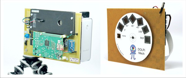
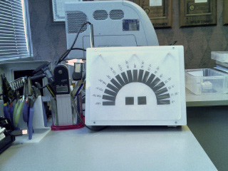
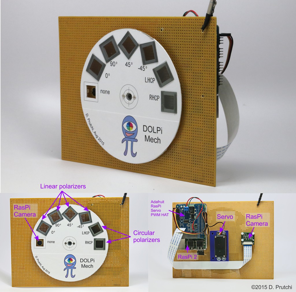
DOLPi_Mech: A Slower But Accurate Imaging Polarimeter
08/24/2015 at 16:18 • 0 comments![]()
The image that the liquid-crystal-panel-based DOLPi takes at "45 degrees" is not strictly that, which is why I state in the paper:
"Bossa Nova’s method is straightforward if laboratory optical-grade components are used. These are very expensive and out of reach for most private enthusiasts. However, I found through experimentation that a welding mask LCP and a polarizer sheet can also give very satisfactory results."
In reality, the LCP driven half-way acts as a quarter-wave plate, and hence the strict interpretation of the analysis at this level is for circular polarization rather than linear polarization at 45 degrees.
I didn't want to go into a thorough explanation of polarization optics to keep the project accessible, but based on my experiments, I'm convinced that DOLPi's "45 degree image" indeed contains a dominant 45 degree component when observing linearly polarized light.
This weekend I decided to build a mechanical filter-wheel-based polarimetric camera to serve as a basis for comparison to the LCP_based DOLPi. This camera is much slower than the LCP-based DOLPi because of the mechanical switching of filters, but it provides the data necessary for complete Stokes imaging (including the fourth Stokes parameter describing circular polarization). The pictures that it produces are of excellent quality!
The camera is also very simple to build, and its operation is simple to understand, so I'll include it within the next version of the project's whitepaper, as well as to the next-stage submission for the Hackaday Prize.
By way of a short explanation, a filter wheel (made of cardboard) holds 6 polarizer filters. Four of them are made of linear polarizer film set so to analyze the image at 0, 90, 45, and -45 degrees when the selected filter is placed in front of the Raspberry Pi camera. The other two filters are circular polarizer films taken from RealD 3D glasses. One slot in the filter wheel is left blank to make it possible to take unfiltered snapshots.
The filter wheel is rotated by a standard servo driven from an Adafruit Servo PWM HAT connected to a RasPi2. The Python code (to be published soon) takes 6 images (although only 4 are really required) to produce a complete Stokes and polarization analysis panel.
DOLPi - RasPi Polarization Camera
A polarimetric imager to locate landmines, detect invisible pollutants, identify cancerous tissues, and maybe even observe cloaked UFOs!