-
1Step 1
Choosing the right object to scan
As every 3D scanning technique photogrammetry has certain restrictions that you need to know before you start scanning. The first program that we use ist VisualSFM. It takes a series of images and creates a 3D point cloud from them. The problem VisualSFM solves while creating the point cloud is called structure from motion.
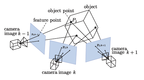
![]() Source: [openmvg.readthedocs.org/en/latest/_images/structureFromMotion.png]
Source: [openmvg.readthedocs.org/en/latest/_images/structureFromMotion.png]As shown in the picture above points on the object are seen by multiple cameras and are saved in the individual images as feature points. The camera may be a single camera moved around a still object taking multiple photos or a group of cameras taking photos at the exact same time. By recognizing object points in mulitple photos both the position of the object points, as well as the position of the cameras, while taking the photos can be calculated.
This leads to the question, what qualifies as a object point and can be detected as a feature point?
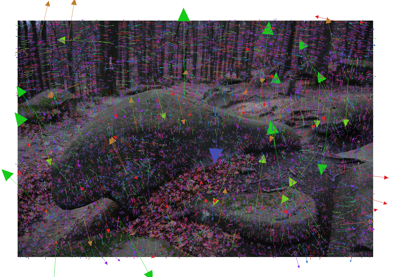
Source:[Alexander Kroth]
The image above shows what the SIFT algorithm, used by VisualSFM, sees in a photo. The arrows are figures of the feature points. A feature point is described by a direction and a magnitude by the SIFT algorithm. It can be seen, that there are a few strong features and many weak ones. The magnitude describes the ability of a feautre point to be recognized in a different photo.
The photo shows a couple of rocks inside a forest with leaves on the ground. A rock is nearly perfect for photogrammetry. It has little to no reflections and very textured. These are already the key requirements for photogrammetry.
- The object needs a certain amount of texture. A white paper or a white wall are very difficult to scan because the algorithm can't find points which are recognizable. Think of the feature points like stars for sailors, it's the same principle. The same problem occurs if you try to scan a textured surface, but the texture can't be captured due to your cameras resolution. Keep that in mind, that your eyes might see texture, your camera won't capture.
- Reflection or transparency should be avoided. The algorithm relies on the fact, that the object won't change from picture to picture and object points stay where they are in the real world. If you stand in front of a mirror and move to the side your reflection moves as well. The problem is, that a object point next to the mirror won't move accordingly. The same applies for reflections on cars etc. The reflection moves with the camera movement and therefore should be avoided. The usual approach of painting the surface with a dull color won't work because you won't have enough texture in that area.
To conclude this chapter here are some examples that work well with photogrammetry and some that might create problems:
Working well:
- Natural stone
- Trees
- Ground (Streets, paths, etc.)
- Fruit (apples)
- Buildings on a larger scale (complete building and not for example a single wall)
- Car interior (depending on the surface, polished surfaces are hard to capture, but the normal plastic surfaces with a bit of roughness work well)
Difficult objects:
- Car exterior (little to no texture, shiny surfaces, glas, reflections.... quite difficult)
- Rooms (large areas like walls without texture)
As mentioned above the algorithm doesn't like movement of objects within the scenery that you try to scan. Therefore nature and crowded spaces are hard to scan. Trees and bushes are quite non-stationary as leaves and branches move. It's ok to capture a tree from a distance, so that little movements are not visible to the camera, but close ups are difficult. As well as trees, people and cars in public spaces tend to move and with them the object points on them, therefore you should avoid to capture pedestrians and moving cars, while trying to scan a building for example.
-
2Step 2
Capture the world properly
In the previous chapter I gave a short introduction in the properties necessary for capturing an object. In this chapter I'd like to describe how to shoot photos for the later use in VisualSFM.
As in photography you don't want areas that are overexposed or underexposed. If you can't lit the object homogenous then it's better to underexpose certain areas than to overexpose. Underexposed areas offer no texture and therefore there are fewer feature points, while overexposed areas tend to show little sparkles, which might create false positives. False positives are, in this context, object points, that are found by the algorithm, but don't exist in the real world. Another important point is to take sharp pictures without motion blur.
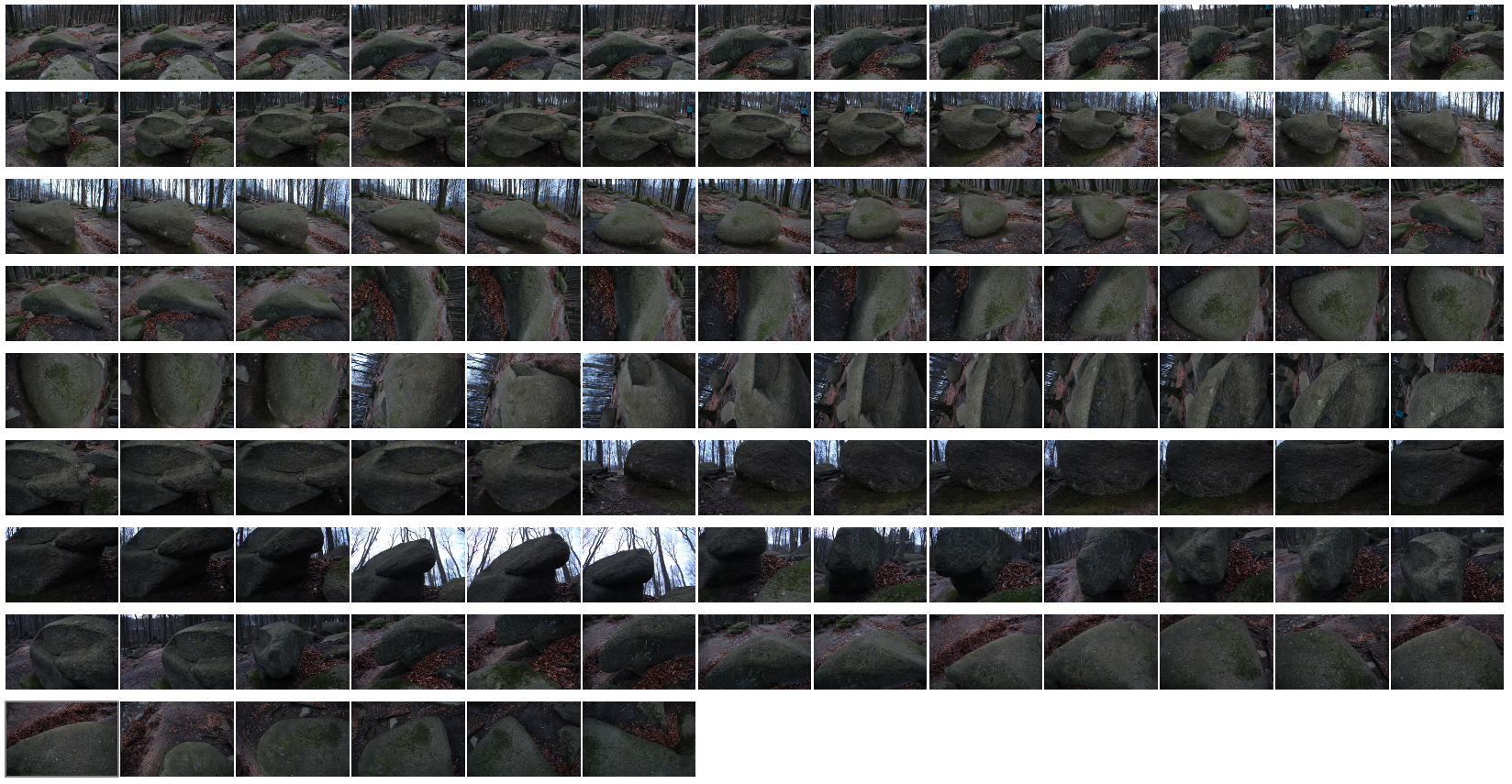
Source:[Alexander Kroth]
The SIFT Algorithm used by VisualSFM detects object points in multiple images. To achieve this the algorithm must fulfill certain requirements. Object points should be found with the following changes from one picture to the other picture: Position/orientation, light, scale.
- Position/orientation: An object point should be recognized in all pictures while you move around him. Imagine it as seeing and recognizing a light switch on the wall from different positions and orientations, while keeping the distance from the light switch.
- Light: Object points should be recognized even if their light conditions change. Keeping the light switch example you should recognize a light switch wether a room is well lit or nearly dark.
- Scale: Object points should be recognized while their size inside the picture changes. For the light switch example this means, that you recognize the same light switch from 1, 5, 10 meters distance.
Knowing these basic principles, how can we optimize our pictures for the algorithm?
As you can see in the image above I've moved around the stone bit by bit, taking images with only a small change in perspective from picture to picture. By this we help the algorithm keeping the factor positon/orientation in good condition. Even though the algorithm can detect object points in two images with a huge difference in perspective, it is better to create a series of images, with only small changes in perspective to achieve more correctly recognized object points and therefore a denser point cloud. Mixing horizontal and vertical pictures doesn't seem to be a problem and won't affect the matching process. Matching is the process of comparing two feature points and deciding wether they represent the same object point in the real world.
If you have the time it's allways better to take more photos. You now might think of using a movie for structure from motion. It works, but you have to keep in mind a few more things, which i might explain in an additional project.
The light conditions in the pictures above are pretty perfect for outdoor structure from motion. A foggy sky with indirect sunlight. Clouds tend to move and... you know. The light conditions should be homogenous with little direct light. I wouldn't recommend using the flash because it's easy to create little overexposures which create false positives and the flash is depended of the current position of the camera, therefore you create quite different light conditions from picture to picture. It's better to use a stationary lamp and think about light before starting to capture photos.
The last point mentioned is scale. With the rock above you might want to capture the rock as a whole and then capture some details on certain parts of the rock. Simply taking a series of pictures from a distance and then taking some close up pictures won't work. As mentioned earlier your camera might not see the texture from the distance, that you can see. Therefore the camera won't see the object points within the details that you try to capture from the distance. It's better to create a series of picture moving towards the detail and from the detail, giving some "guide" to the algorithm. To capture multiple parts of an object and even details it is good to think of taking pictures in a flow. Don't interrupt taking pictures and only make small changes in perspective from picture to picture.
-
3Step 3
Preheat your GPU, we're starting VisualSFM
In the steps before we discussed the principles of taking suitable pictures. Now we create a point cloud based on those pictures. First download and unzip VisualSFM. If you have a recent Nvidia GPU chose the 64bit CUDA version. CUDA is a framework for parallel processing on GPUs and makes the process of matching images notably faster (10x or more...). Now download the CMV program and unzip it in the same folder als VisualSFM.
Source:[Alexander Kroth]
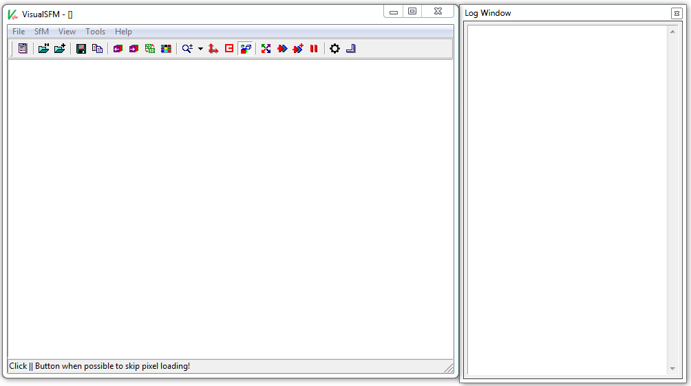
In this tutorial I will only explain the buttons necessary. VisualSFM offers many options for optimization and different view options, but only the ones necessary will be covered. To enable GPU processing choose Tools->Enable GPU->Standard Param and Tools->Enable GPU->Match using CUDA. If you don't have CUDA available you have to check Tools->Enable GPU->Disable SiftGPU and Tools->Enable GPU->Match using GLSL.
Click on File->Open+ Multi Images. Now choose all images that you want to process and open them. Note that, when opening large numbers of files (500+), VisualSFM sometimes crashes or won't load any images at all. You can view the pictures now by clicking and dragging or zoom in.
Once all images have been loaded, which can take some time, depending on the image size, we want to detect and match the feature points of the given images. First click on SfM->Pairwise Matching->Show Match Matrix. The same view can be accessed by clicking on the colored tiles symbol while holding shift. Now all images are shown on both the x- and y-axis. Now choose SfM->Pairwise Matching->Compute Missing Match.
Source:[Alexander Kroth]
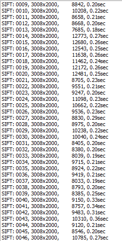
VisualSFM now starts to apply the SIFT algorithm to every image. The picture above shows the output for a series of pictures. The last column is the time needed to find all feature points in the picture. The one before gives you the numer of feature points found in a picture. A low number of feature points means that the SIFT algorithm couldn't find many recognizable object points in the picture. You should aim for a high number of feature points for matching.
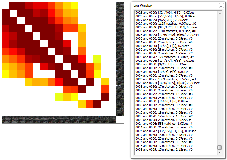
Source:[Alexander Kroth]After finding all feature points VisualSFM starts to match the feature points against each other to find object points visible in multiple pictures. The diagonal of the matrix would mean an image is matched against itself. As there is no use in doing that, the diagonal stays white, which means, that no matches or very little have been found. A dark red color represents a high number of matching feature points while yellow and green represent a lower number of matching feature points. The log windows shows the number of matches for a pair of images and the time taken to compute these. Note that both computing the SIFT features and matching the features is VERY demanding for your hardware, therefore you shouldn't be working on the pc while it is matching.
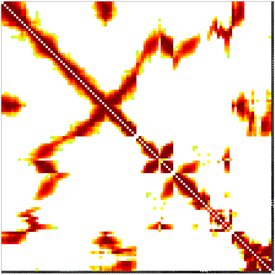
Source:[Alexander Kroth]Be patient while matching, depending on the picture size and the number of pictures it takes from minutes to hours to complete.You can stop the matching process with Ctrl+C, but be warned that VisualSFM tends to crash if matching is stopped. If this happens simply restart the program and open your pictures again. VisualSFM keeps track of the sift features and matches already found. The image above shows a finished matching process. You can now see how the pictures are matched. If you draw a horizontal line from one of the pictures on the right side you can see als pictures that have matching feature points on the buttom of the matrix. If you have small islands inside this picture with nothing horizontally or verticaly from it, these images tend to create seperated point clouds not connected the main one.
Additional Information:
If you have a series of pictures that don't form any loops, for example you walk in a straigt line for a while, while taking pictures in contrary to walking in circles, you won't need to match a picture, taken hundreds of meters away from another picture, with said picture. For this occasion you can use SfM->Pairwise Matchin->Compute Sequence Match. VisualSFM only matches pictures within a given range. For exmaple 10 pictures before and after a picture. Keep in mind to name the pictures according to their logical order, for example first picture of a path is 1 and the last one is 900 with increasing numbers.
-
4Step 4
Time to change the dimension, calculating point cloud
After sucessfully matching all images we now can create the point cloud
Source:[Alexander Kroth]
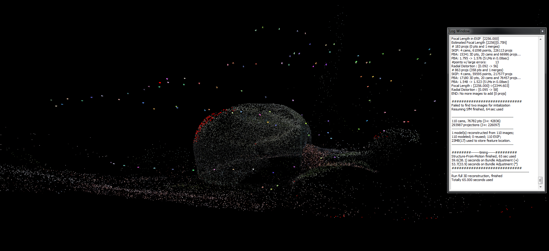
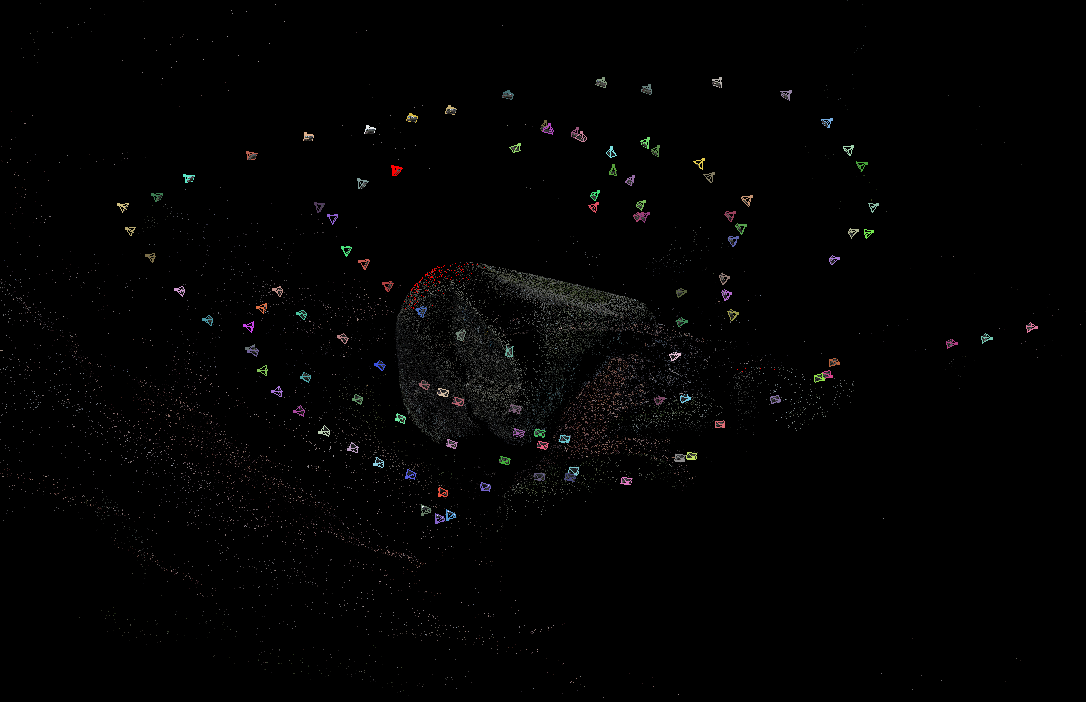
To give you an idead of how long it takes to detect the feature points and to match them: A series of 110 pictures, shown above, with an image size of 3008x2000 pixels and a number of features per picture of around 6000 to 10.000 takes about 16 seconds to find all feature points. The matching takes another 10 minutes. Note that these values apply for matching and feature detection performend on a GPU.
After the match matrix has been filled, we now can start to compute the point cloud. It is possible to stop matching and compute the pointcloud with only a part of the pictures matched, if you want to see if the pictures sucessfully form a point cloud.
To compute the point cloud click on SfM->Reconstruct Sparse. VisualSFM now places the cameras and objects points. To pan the view use the left mouse button and to rotate the view use the right mouse button. By holding Shift and scrolling you can increase or decrease the point size. By holding Ctrl and scrolling you can increase the size of the cameras. If the center of rotation is shifted outside the model you can use the coordinate system symbol in the upper bar to recenter it.
To improve the point cloud click on SfM->More Functions->Bunde Adjustment.
Additional Information:
VisualSFM tries to create a single point cloud out of the given picture set. If it fails to do so, multiple point clouds will be created. To show multiple created point clouds click on View->Show Single Model. To change the current point cloud click on View->Next Photo/Pair while seeing multiple point clouds. To switch back to a single point cloud click on View->Show Single Model.
You might want to scan an object with light colors and it may be hard to see those points in the point cloud. You can switch to a dark background with View->Dark Background
-
5Step 5
Denser Point Clouds ahead! - CMVS
After the preceding step we have created a point cloud.
Source:[Alexander Kroth]
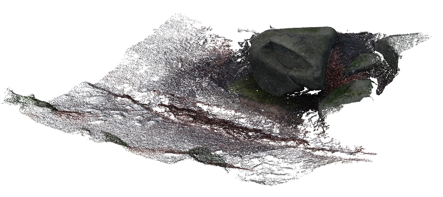
Based on this point cloud we can create a denser point cloud using CMVS. CMVS takes the point cloud created in VisualSFM and applies a multi-view stereo algorithm. I contrary to Structure from Motion CMVS takes to camera views which are nearly parallel and estimates the depth of the scene based on the stereo view, simliar to the human vision. CMVS uses the existing point cloud and applies a depth map onto the exisiting point cloud forming a denser point cloud. While the density of the point cloud increases you get more errors, mostly at rough edges or in poorly covered areas of the object. If you have taken enough pictures and the point cloud from VisualSFM already contains many points then CMVS will work really well. Be warned that CMVS takes extremly long to compute depending on the number of pictures and the picture size.
To compute the CMVS point cloud click on SfM->Reconstruct Dense. Choose a folder name for the dense point cloud and the computation will begin.
Source:[Alexander Kroth]
By comparing both images you already see the difference. CMVS is needed to later apply a texture to an object in meshlab. As you can see from the number of words in the first chapters in comaprision to this chapter the possibilities to take influence on the process get smaller. So it is important to take care with the first steps and the later steps will work better.
-
6Step 6
A brief introduction to Meshlab
The next step after creating a dense point cloud is to create a mesh. We use Meshlab for this purpose. For the next steps it's important to note, what CMVS creates besides the dense point cloud. CMVS saves all camera positions to a file and creates a list of already alligned images for texturing.
Source:[Alexander Kroth]
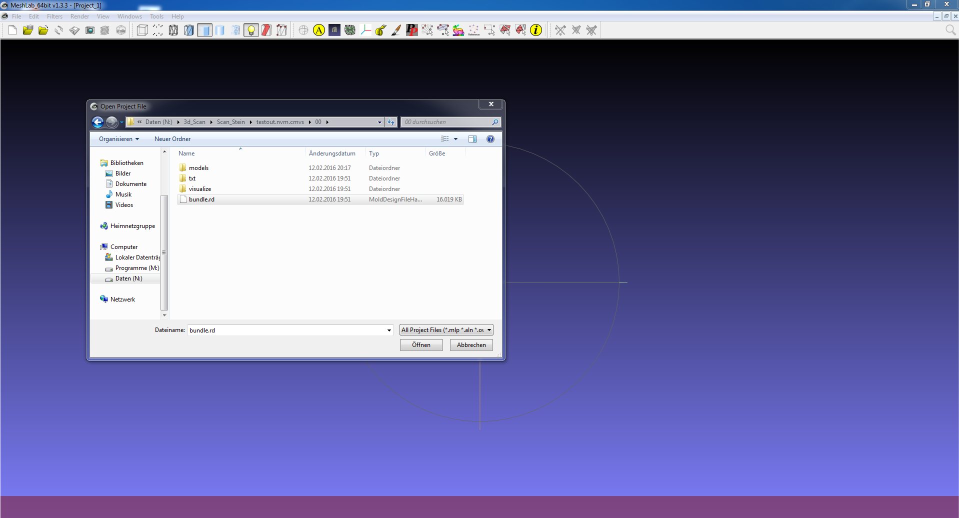
Downloading and installing Meshlab shouldn't make any trouble, therefore we directly start with opening our project. Click on File->Open Project. Now choose the folder which CMVS created while creating the dense point cloud. Within the folder, here named testout.nvm.cmvs, is a folder 00. There may be more folders, depending on the number of processed models. CMVS can process all point clouds that VisualSFM found from a picture set in series, therefore more than one folder may be created. Choose the folder according to the model you want to load into Meshlab, mostly it's 00. Within 00 is a bundle.rd file, which we choose. Now Meshlab asks for a file containing a list of images. It's in the same folder named list. After choosing both files Meshlab starts to load the point cloud, the images for texturing and the camera positions.
The camera controls in Meshlab are different from the camera controls in VisualSFM. Left click is used for rotating, clicking the mouse wheel pans the point cloud and zooming is possible by scrolling. To recenter the center of rotation double click on the desired point. The first thing to do after starting Meshlab is to open the Layer Dialog. You can either open the Layer Dialog by pressing Ctrl + L or clicking on View->Show Layer Dialog.
Source:[Alexander Kroth]
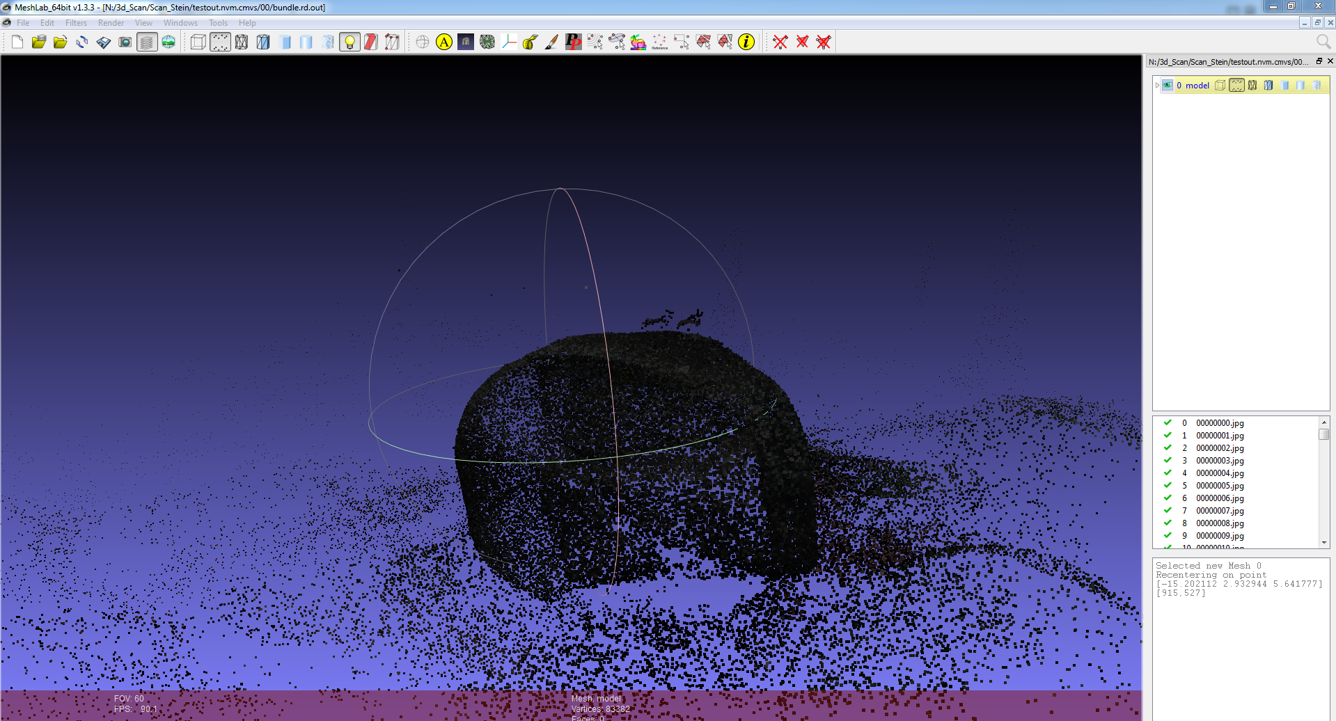
As you can see in the image above it's important to keep in mind that everything thats on the initital pictures might slip into the final pointcloud. Here we can see my feet standing on top of the stone, which I accidently captured while photographing the top of the stone.
On the right of the image you can see the Layer Dialog. The bundle.rd file already contained the point cloud, which is shown as 0 model. You can either hide the model from view or choose wether points, wireframe or different versions of the mesh are displayed. While executing operations in Meshlab keep in mind that operations are only applied to the choosen models in the Layer Dialog. It's also extremely important to note, that Meshlab has no Undo Button! Meshlab mostly works by creating new layers, while applying filters, but once you delete for example points from a point cloud they are gone. It's a good idead to save your work once in a while and to copy a layer and work on the copy to keep the original data while in Meshlab. Meshlab tends to crash from time to time, so there's another reason for saving regular.
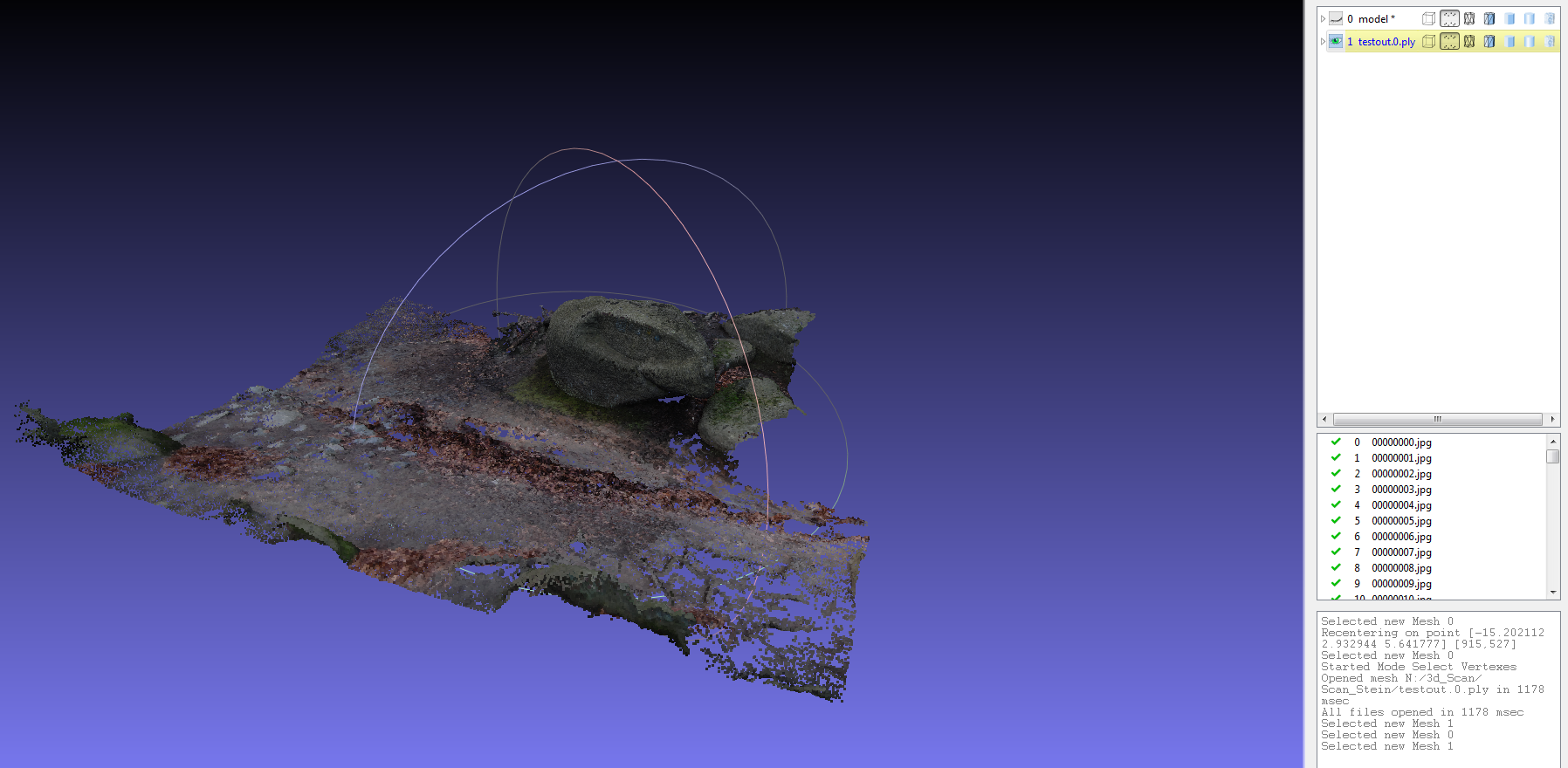
For the further process we won't use the point cloud given by CMVS. Click on File->Import Mesh and choose the .ply file created by CMVS, which is in the same folder as the CMVS folder. In the given case it would be a testout.ply file next to the testout.nvm.cmvs folder. Choose the .ply file and load the point cloud to Meshlab.
Source:[Alexander Kroth]
The Layer Dialog should now contain the initial point cloud and the dense point cloud. I've hidden the initial point cloud in the image above and already cleaned unnecessary parts of the point cloud
Once we have all necessary point clouds loaded into Meshlab it's time to clean up those point clouds.
Source:[Alexander Kroth]
Most point clouds are not ready to create a mesh directly from the data given by VisualSFM. Therefore we need to delete unnecessary parts of the point cloud. The image above shows the necessary buttons. The selected button let's you choose the points to be deleted. It only offers a rectengular selection. To delete the selected points choose the button, showing the three dots connected by lines, on the right.
After cleaning our point cloud we can now proceed to calculating the normals.
-
7Step 7
Calculating normals in Meshlab
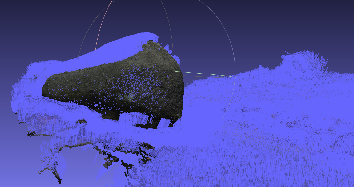
In the following step we will apply the Poisson Filter to the point cloud to create the mesh. The Poisson Filter requires every point of the point cloud to have a vector assigned. The vector is the normal vector for a plane through that point. It describes the orientation and the direction of the plane. The normal vector points outwards, so it stands on top of the mesh and faces away from it.
Normally CMVS already creates normal vectors that are aligned correctly, but in some point clouds some parts fail to generate correct normal vectors.
Source:[Alexander Kroth]
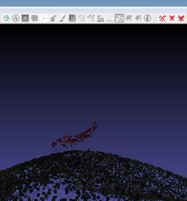
This problem is caused by the CMVS output. The CMVS bundles a set of fotos with nearly the same orientation and calculates "stereo images". It might happen that there a two valid solution for the surface orientation and therefore the normals are flipped. We have to import single CMVS outputs instead of the already assembled dense point cloud. Follow the steps for opening a pointcloud in Meshlab like discribed in the chapter before until the step where the dense point cloud is opened. Instead of importing the .ply file in the main folder head to the folder where you imported the bundle.rd. There open the models folder and open all option-000x.ply files. These contain the different CMVS outputs. Now we can toggle single point cloud on and off to see which part is flipped. [I'm writing a small program to flip normals in the .ply format, which seems not possible in Meshlab. With the corrected normals you can simply follow the next steps] To flip the normals in the .ply file, just open them with the program in my github. After correcting the normals open the single point clouds again in Meshlab like described before. Note that the dense point cloud, which contains all CMVS outputs wasn't corrected, so it is necessary to import the single files.
[Image points cloud on the right]
Source:[Alexander Kroth]
For the next steps we will need a single point cloud containing all CMVS outputs. The first pointcloud in Meshlab, representing the output of VisualSFM, can be deleted (right click on the entry on the right and choose Delete Current Mesh) or set invisible. To merge all CMVS output set all of them visible and right click on the lowest in the list. Now choose Flatten Visible Layers and check Merge Only Visible Layers and Keep unreferenced vertices. The first option can be used to choose which point clouds should be merged and the second option is needed to prevent Meshlab from deleting the point clouds.
Wether we already had a correct dense point cloud or not we now can proceed to create a mesh from this point cloud.
-
8Step 8
Poisson Filter for the transition from point cloud to mesh
Meshlab offers three different filters to calculate a mesh. From my experience the Poisson Filter gives the best solution, but requires normals. In case you have to handle a point cloud without normals you can still use the Ball Pivoting Filter.
Start the Poisson Filter by clicking Filters->Point Set->Surface Reconstruction: Poisson.
-
9Step 9
Preparing a high poly mesh for Meshmixer
-
10Step 10
Creating a watertight STL in Meshmixer
Photogrammetry 3D Scanning
This project is a brief tutorial from acquiring multiple images to a finished 3D print of a real world object.
 Source: [
Discussions
Become a Hackaday.io Member
Create an account to leave a comment. Already have an account? Log In.
Hi. Thanks for the clear explanation of visual SFM. now I am working with visual SFM and I have some questions about it. I was wondering if you can help me to figure out those questions answer.
Are you sure? yes | no