 Brett Smith
-
Raspberry Pi Zero: Controller Loop Stability
02/07/2019 at 12:52 • 0 commentsRaspberry Pi Zero: Controller Timing Stability
Servo motor control is usually implemented with an embedded MCU as typically very fast, consistant control loops are required for real life motion controls. Programming, capturing data, and PID tuning can be tedious in an embedded system environment. So in this notebook we will be examining raspberry pi zero loop stability while controlling a brushed, dc motor.We will be testing the loop timing under different conditions:
1) Executing normally
2) Executing as an individual python thread
3) Executing during video streaming
4) Executing with multiple controller threads
5) Executing with overclocked CPUProcedure
Because this platform is ultmately being developed for a raspbery pi robot with a live video stream using gstreamer, I will test the loop time both while the raspberry pi is streaming and not streaming video. A total of 8 tests were performed in a variety of combinations of the above conditions. Those conditions can be seen in the table below:
We will build a list of execution times for each testing state and analyze the distribution of those execution times. This will enable us to analyze the frequency and stability of the control loop.Video Not Streaming Video Streaming Overclocked CPU: Video Not Streaming Main Loop Test 1 Test 3 Test 7 Threaded Loop Test 2 Test 4 Test 8 5 Threaded Controllers Not Tested Test 5 Test 9 2 Threaded Controllers Not Tested Test 6 Test 10 Software
The raspberry pi is using berryconda to manage python virtual environments, and is running a native jupyter notebook server to allow quick code editing and easy data capture.
Hardware
Between the raspberry pi there is a micrcontroller and an h-bridge. The microcontroller is setup to measure encoder counts and send them when requested to the Raspberry Pi. Likewise, the microcontroller listens to the serial line and sets the motor direction and PWM based off raspberry pi commands.
![IMG-20190207-142511]() In [43]:
In [43]:#! /home/pi/berryconda3/envs/pidtuner/bin/python %matplotlib inline import matplotlib import seaborn as sns import matplotlib.pyplot as plt import serial import time import RPi.GPIO as GPIO import atexit import random import threading import numpy as np from scipy.stats import norm from scipy import stats
In [3]:ser = serial.Serial( port = '/dev/ttyS0', baudrate = 115200, bytesize = serial.EIGHTBITS, parity = serial.PARITY_NONE, stopbits = serial.STOPBITS_ONE, timeout = 1, xonxoff = False, rtscts = False, dsrdtr = False, writeTimeout = 2 )
In [4]:def setPwm(pwm): message = str.encode('R' + str(pwm) + '!') ser.write(message) def getRevs(): ser.write(str.encode('?!')) val = ser.readline() return (int(val))
In [5]:class PID (threading.Thread): setpoint = 0 last = 0 error = 0 lastValue = 0 Tkp = 0 Tki = 0 Tkd = 0 def __init__(self, kp, ki, kd, direction, outputFunc, inputFunc, threadID): threading.Thread.__init__(self) self.kp = kp self.ki = ki self.kd = kd self.direction = direction self.threadID = threadID self.outputFunc = outputFunc self.inputFunc = inputFunc self.output = 0 #Used for thread timing self.count = 0 self.runtimes = [] #This is used to terminate the thread self.shutdown_flag = threading.Event() self.min = 0 self.max = 0 def join(self, timeout=None): self.shutdown_flag.set() threading.Thread.join(self, timeout) def setLimits(self, outputMin, outputMax): self.min = outputMin self.max = outputMax def __run__(self): controllerInput = self.inputFunc() controllerOutput = self.compute(controllerInput) self.outputFunc(controllerOutput) def run(self): while not self.shutdown_flag.is_set(): #self.__run__() dt = self.timeFunc(self.__run__) self.runtimes.append(dt) self.count += 1 def timeFunc(self, func): start = time.monotonic() func() return time.monotonic() - start def compute(self, value): #update timer now = time.monotonic() dt = now - self.last self.last = now #update PID terms self.error = self.setpoint - value self.Tkp = self.kp*self.error self.Tki += self.ki*self.error*dt self.Tkd = self.kd*(value - self.lastValue)/dt self.lastValue = value output = self.Tkp + self.Tki - self.Tkd if output < self.min: output = self.min if output > self.max: output = self.max self.output = output*self.direction return(self.output)
In [6]:pid1 = PID(17,0,0.16, -1.0, setPwm, getRevs, 'pid1') pid1.setLimits(-1000.0, 1000.0) pid1.setpoint = getRevs() @atexit.register def exit(): setPwm(0.0) pid1.shutdown_flag.set() pid1.join() ser.close() GPIO.cleanup() print('PID test ended.')
Test 1: Main Loop Execution, No Video Stream
In [7]:def mainTest(): count = 0 main_loop_times = [] pid1.setpoint = getRevs() - 625 while count < 1000: now = time.monotonic() pid1.__run__() main_loop_times.append(time.monotonic() - now) count += 1 setPwm(0.0) return main_loop_times
In [37]:data1 = mainTest() mu, std = norm.fit(data1) sns.distplot(data1) print('Mean',mu) print('Standard Deviation', std) print('Number Samples', len(data1)) fig = plt.figure() ax = fig.add_subplot(111) stats.probplot(data1, dist=stats.loggamma, sparams=(2.5,), plot=ax) plt.show()
Test 2: Threaded Execution, No Video Stream
In [9]:def threadTest(): pid = PID(17,0,0.16, -1.0, setPwm, getRevs, 'pid1') pid.setLimits(-1000.0, 1000.0) pid.setpoint = getRevs() - 625 count = 0 thread_loop_times = [] pid.start() while(pid.count < 1000): time.sleep(0.01) pid.shutdown_flag.set() pid.join() return pid.runtimes
In [38]:data2 = threadTest() mu, std = norm.fit(data2) sns.distplot(data2) print('Mean',mu) print('Standard Deviation', std) print('Number Samples', len(data2)) fig = plt.figure() ax = fig.add_subplot(111) stats.probplot(data2, dist=stats.loggamma, sparams=(2.5,), plot=ax) plt.show()
Test 3: Main Loop Execution, Video Streaming
In [13]:data3 = mainTest() mu, std = norm.fit(data3) plt.hist(data3, bins=100, density=True, color='g') plt.show() print('Mean',mu) print('Standard Deviation', std) print(len(data3))
Test 4: Threaded Execution, Video Streaming
In [14]:data4 = threadTest() mu, std = norm.fit(data4) plt.hist(data4, bins=100, density=True, color='g') plt.show() print('Mean',mu) print('Standard Deviation', std)
Test 5: 5 Threaded Execution: Video Streaming
In [33]:def fakeFoo(var): return 0 def fakeFoo2(): return 0
In [31]:def multiThreadTest(numThreads, waitCounts): pids = [] data = [] count = 0 pid = None pid = PID(2,0,0.0, -1.0, setPwm, getRevs, 'pid'+str(count)) pid.setLimits(-1000.0, 1000.0) pid.setpoint = getRevs() - 625 pids.append(pid) count += 1 while(count < numThreads): pid = None pid = PID(17,0,0.16, -1.0, fakeFoo, fakeFoo2, 'pid'+str(count)) pid.setLimits(-1000.0, 1000.0) pid.setpoint = getRevs() - 625 pids.append(pid) count += 1 for pid in pids: pid.start() print('Threads Spawned') while(pids[0].count < waitCounts): time.sleep(0.01) print('Done Waiting') for pid in pids: pid.shutdown_flag.set() pid.join() print('Threads shutdown') for pid in pids: data += pid.runtimes setPwm(0.0) return pids[0].runtimes
In [36]:data = multiThreadTest(5,100) mu, std = norm.fit(data) sns.distplot(data) print('Mean',mu) print('Standard Deviation', std) print('Number Samples', len(data)) fig = plt.figure() ax = fig.add_subplot(111) stats.probplot(data, dist=stats.loggamma, sparams=(2.5,), plot=ax) plt.show()
The running time is almost 10x greater spawing 5 of the threads! This greatly affects controller performance. According to 'top' this program was occupying 85% of CPU overhead. Although even single threaded tasks seem to occupy this much overhead.
Test 6: 2 Threaded Execution, Video Streaming
In [35]:data = multiThreadTest(2,1000) mu, std = norm.fit(data) sns.distplot(data) print('Mean',mu) print('Standard Deviation', std) print('Number Samples', len(data)) fig = plt.figure() ax = fig.add_subplot(111) stats.probplot(data, dist=stats.loggamma, sparams=(2.5,), plot=ax) plt.show()
Two threads (which we will need) has much better loop time although the CPU overhead is still comparable.
Pi Overclocked to 800 MHz
I wasn't thrilled with the update rate of the control loop, and the amount of processor overhead, so I tried overclocking the pi from 700 MHz to 800 MHz
Test 7: Pi Overclocked, Main Thread, No Video Stream
In [25]:## Main Thread : No Video Stream data5 = mainTest() mu, std = norm.fit(data5) sns.distplot(data5) print('Mean',mu) print('Standard Deviation', std) print(len(data5)) fig = plt.figure() ax = fig.add_subplot(111) stats.probplot(data5, dist=stats.loggamma, sparams=(2.5,), plot=ax) plt.show()
Test 8: Pi Overclocked, Threaded Execution, No Video Stream
In [40]:## Threaded: No Video Stream data6 = threadTest() mu, std = norm.fit(data6) sns.distplot(data6) print('Mean',mu) print('Standard Deviation', std) print('Number Samples', len(data6)) fig = plt.figure() ax = fig.add_subplot(111) stats.probplot(data6, dist=stats.loggamma, sparams=(2.5,), plot=ax) plt.show()
Test 9: Pi Overclocked, 5 Controller Threads, No Video Stream
In [42]:## 5 Threaded Overclock, No Video Stream data = multiThreadTest(5,100) mu, std = norm.fit(data) sns.distplot(data) print('Mean',mu) print('Standard Deviation', std) print('Number Samples', len(data)) fig = plt.figure() ax = fig.add_subplot(111) stats.probplot(data, dist=stats.loggamma, sparams=(2.5,), plot=ax) plt.show()
Test 10: Pi Overclocked, 2 Controller Threads, No video Stream
In [41]:## 2 Threaded Overclock: No Video Stream data = multiThreadTest(2,1000) mu, std = norm.fit(data) s
Motor Sizing & Wheel Selection
06/05/2018 at 09:10 • 0 commentsHello All!
In this post I am hoping to showcase some of the design work that goes into motor selection. If you are curious about this process, I highly recommend the free resources available at the California Mechatronics Center .This company is actually run by one of my previous university professors and the workflow presented SERIOUSLY cuts down on a lot of mechanical design iteration. The documentation shown here could certainly help you build much more precise CNC/servo systems than I present here (although beam deflection seems to be missing...).
After all was said and done, this process seemed to work out fairly well considering all of the parts are DIY robotics components. It met all of our requirements on the first go!
I did, however, make one glaring mistake:After assembly and testing, the motors could stop so quickly that robot would flip over! Pretty much a catastrophe an industrial scale, but not a big deal with low-mass system such as this. Certainly something to take into account in the future. Rather than programming in a maximum de-acceleration rate, a small counterweight remedied the problem.
So lets dive into it!The primary issue in selecting a motor is ensuring that the motor can meet both of your torque and speed requirements. If you have these specifications before you start, the worst is over! If not, you will have to estimate them yourself.
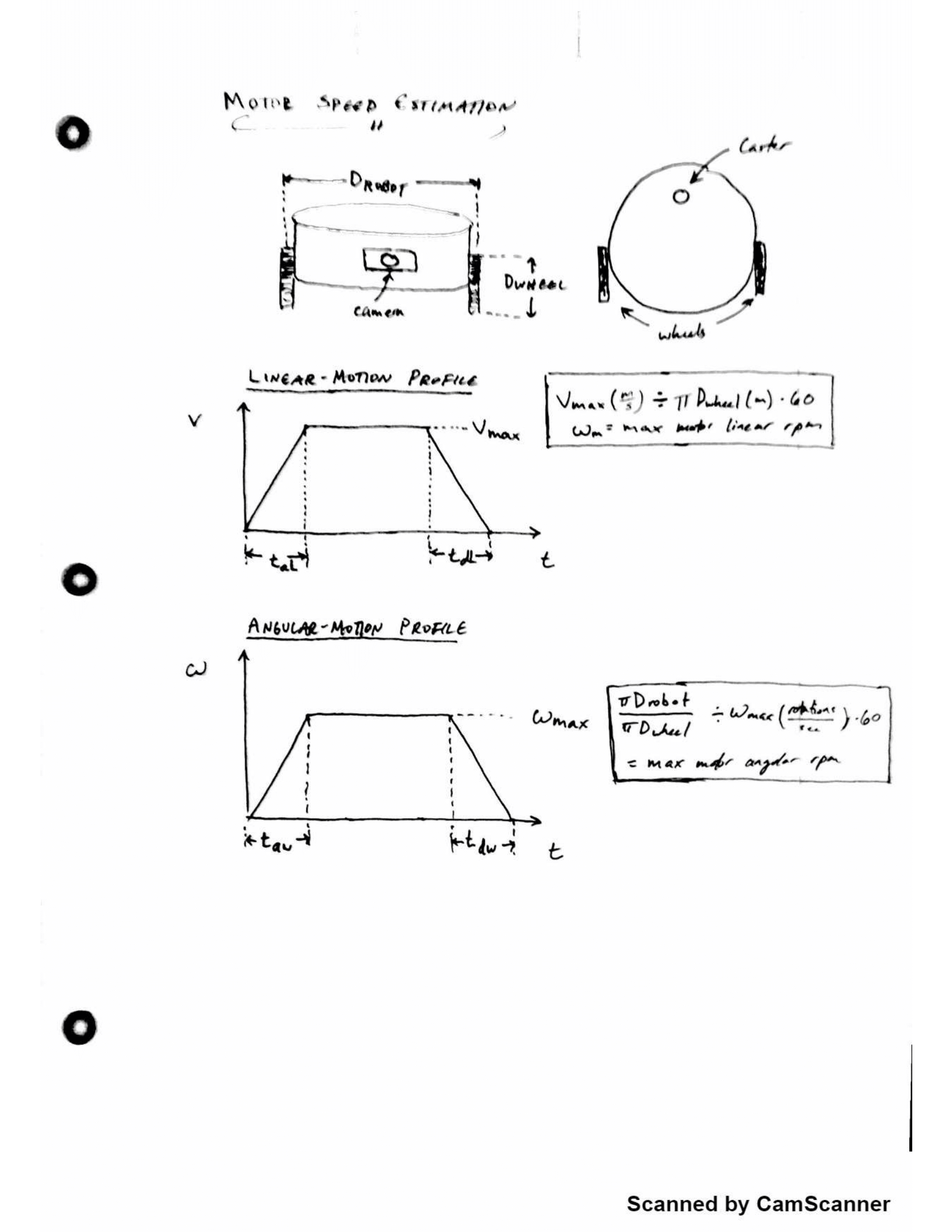
Here is the big boy check list. Seriously, this process separates the engineers from the hobbyists.The first step involves in creating a motion profile for each of your motors. The key here is to find your systems top speed and the amount of time you are allowed for the motors to spin up. This will help you determine the motors required angular acceleration. See below
![]()
Notice that we have created two motion profiles. One helps determine the acceleration required to meet our requirement for the bots linear motion (i.e. forwards and backwards movement), and the other to determine the acceleration to meet the requirements for the bots turning speed (i.e. spinning about its center).
The big design take away from both these graphs (for our project anyway): the relationship between wheel sizes, robot diameter and the maximum required motor velocity.
A smaller diameter robot really cuts down on the acceleration required for turning, and larger wheels will likewise cut down the acceleration required for linear velocity.
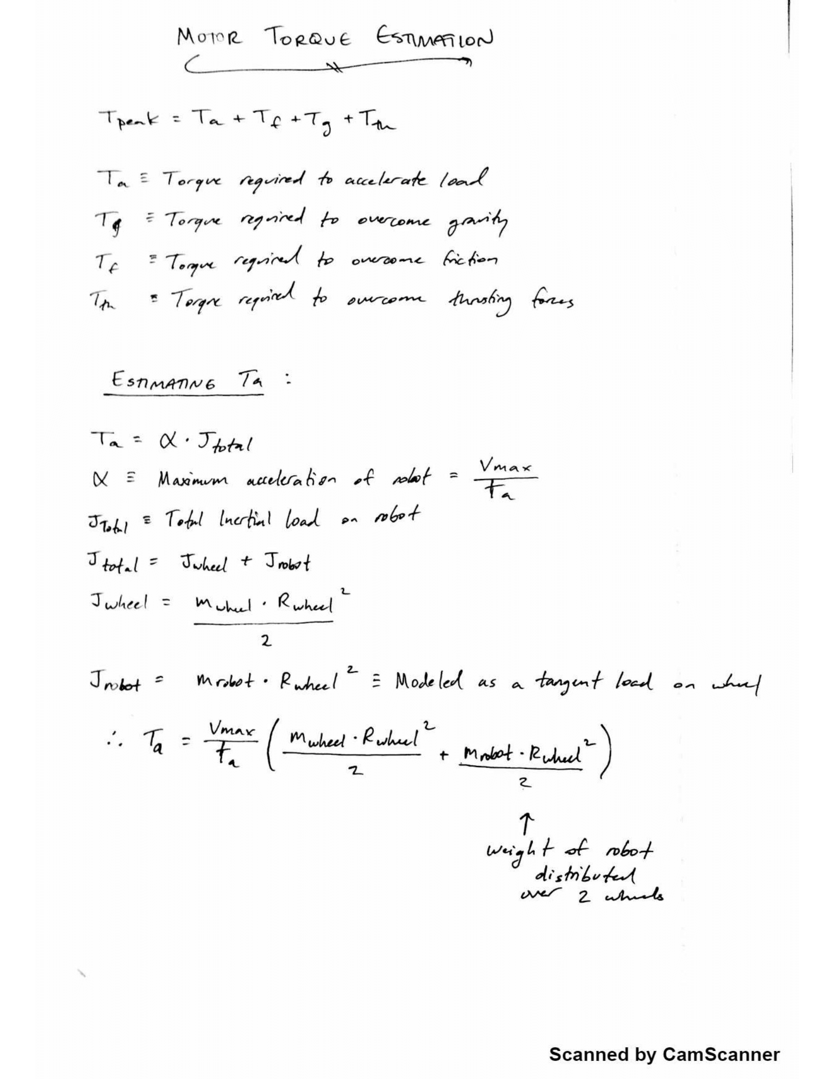
Now that we have our head around that, lets take a look at our kinematics, and calculate our peak torque:![]()
Luckily for me, this system is a simple one:
- There are no major safety hazards if one of the motors fails.
- There are no mechanics (belts, ballscrews) to complicate our calculations -our motor go to a gearbox, and then wheels. These add extra inertia loads and frictional forces to account for.
- Our system is stable even if the motors are not running.
- No shear force on the motor shafts outside the weight of the bot.
So we don't really have to consider much in the way of frictional, gravitational, or thrusting forces.
Pretty easy living! All we have to really determine is the inertia the bot imposes on the motors, which can be treated as tangent load on the edge of each wheel (see the equation for Jrobot).
Tthe main thing to notice is that increasing wheel diameter is not without its drawbacks. While this does decrease the maximum required speed of the motor, it seems to add quite a bit more inertia (notice the inertia exerted by the bot increases with the square of the wheel radius).
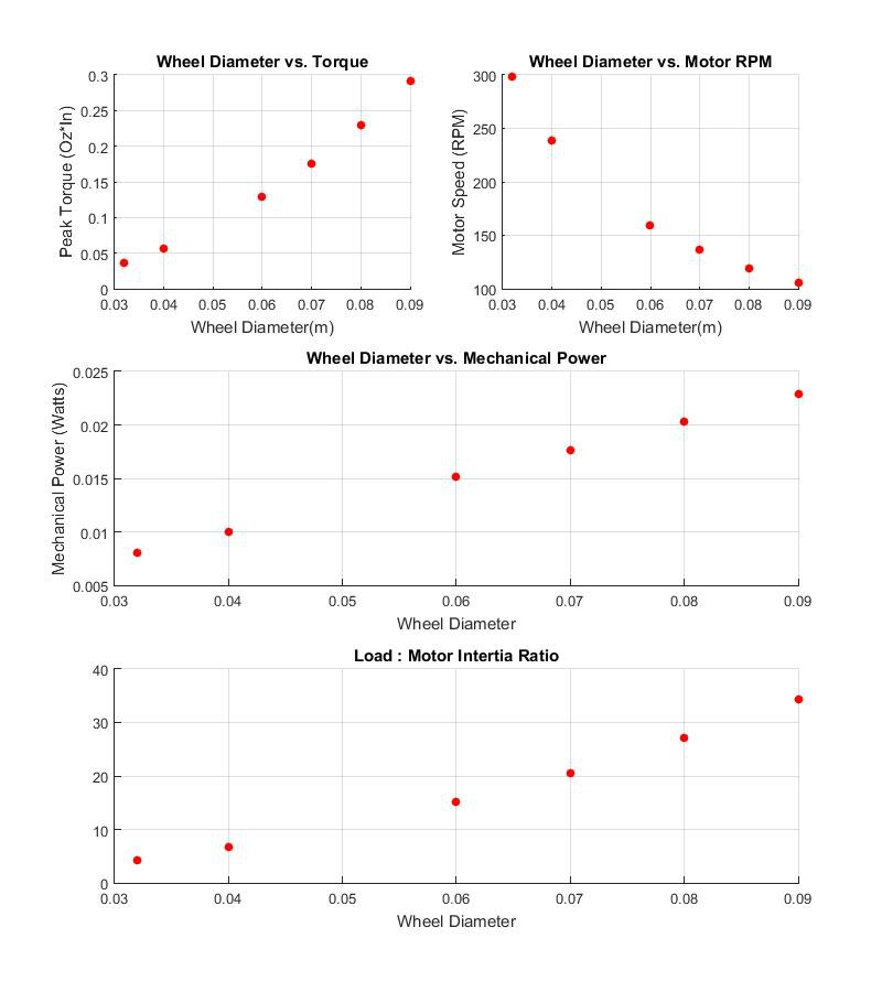
So all that is left is to accurately estimate all of our equation parameters. I use matlab, but this could easily be excel. This will let you tweak each of your design parameters (in our case, bot diameter and wheel diameter). Lets plot all of our motor parameters as they vary with our bot dimensions.
Here is the output of our matlab script:![]()
One parameter that is commonly overlooked is the ratio between motor inertia and load inertia. A lot of discussion here. The rule of thumb in the industry is to never exceed 50:1, but if your a controls whiz you can probably get away with much worse.
One last note, you really don't want to operate exactly at your motors maximum power output. You want your requirements to fall underneath the motors torque-speed curve.
Motor shopping and driver selection to follow!
Here is the matlab script:
Vbot = .5;         % Top linear-speed (m/s)
Abot = 2;           % Minimum linear-acceleration (m/s^2)
Mrobot = .90;      % Mass of robot in Kg
Drobot = 0.15;      % Distance between wheels in M

%Wheel options
Dwheel = [.032,  .04,   .06,    .07,    .08,    .09];
Rwheel = Dwheel/2;
Mwheel = [.0032, .0043, .0114, 0.0141,  0.0198, 0.02267];


%Time to accelerate to Vbot
Ta = Vbot/Abot;

%Top speed of the motor in rpm
Wmotor = Vbot./(pi*Dwheel)*60;

%Inertial Loads

Jwheel = 0.33*Mwheel.*(Rwheel.^2);
Jrobot = 0.5*Mrobot.*Rwheel.^2;
Jload = Jwheel + Jrobot;

%Peak torque
Tpeak = Abot*(Jwheel + Jrobot);

%Calculating Power required:
Mpower = 2*pi*Tpeak.*Wmotor/60;

%Calculating Load:Rotor Inertia Ratio:
Jrotor = 10; %g*cm^2
Gratio = 30; %Gear ratio
Jrotor = Jrotor * 10^-7;

fig = figure;
set(fig, 'Position', [300 100 800 900]);
subplot(3,2,1);
scatter(Dwheel, Tpeak*141.611,'filled','r');
ylabel('Peak Torque (Oz*In)');
xlabel('Wheel Diameter(m)');
title('Wheel Diameter vs. Torque')
grid on;

subplot(3,2,2);
scatter(Dwheel, Wmotor, 'filled','r');
title('Wheel Diameter vs. Motor RPM');
xlabel('Wheel Diameter(m)');
ylabel('Motor Speed (RPM)');
grid on;

subplot(3,2,[3 4]);
scatter(Dwheel, Mpower,'filled', 'r')
title('Wheel Diameter vs. Mechanical Power');
xlabel('Wheel Diameter');
ylabel('Mechanical Power (Watts)');
grid on;

subplot(3,2,[5 6]);
scatter(Dwheel,(Jload/Jrotor)/Gratio,'filled','r');
title('Load : Motor Intertia Ratio');
xlabel('Wheel Diameter');
grid on;
LabRATory Telepresence Robot
This robot moves vicariously for a laboratory mouse while its brain is imaged by a microscope!
