In this video i compare the real robot model with the simulation model:

I'm using PyBullet physics engine, it is simple to use and seems to have a good performance as well as very precise results. In the video you can see that the simulation is a bit slow, this is becouse the simulation (at the time of the video) was not working at real time but computing the simulation every 20 ms.

This log is going to be about the python communication files, explaining the interfaces used in order to communicate both with the ps3 controller and with the arduino.

Serial Bidirectional Communication on python.

This is written in the serial_com.py file and the code goes as follow:

• First thing is to define the serial port and its baudrate.

import serial

class ArduinoSerial: 
    def __init__(self , port):
        #ls -l /dev | grep ACM to identify serial port of the arduino
        self.arduino = serial.Serial(port, 500000, timeout = 1)
        self.arduino.setDTR(False) #force an arduino reset
        time.sleep(1)
        self.arduino.flushInput()
        self.arduino.setDTR(True)

• Then the communication is done with the next two fuctions. This fuctions are very general and can be used without big chnges.

This program will stop the main loop until the next data arrives, this way the arudino memory is not overloaded with the pulse commands arriving.

def serialSend(self, pulse):  
        comando = "<{0}#{1}#{2}#{3}#{4}#{5}#{6}#{7}#{8}#{9}#{10}#{11}>" #Input
        command=comando.format(int(pulse[0]), int(pulse[1]), int(pulse[2]), 
                                   int(pulse[3]), int(pulse[4]), int(pulse[5]), 
                                   int(pulse[6]), int(pulse[7]), int(pulse[8]), 
                                   int(pulse[9]), int(pulse[10]), int(pulse[11]))
        self.arduino.write(bytes(command , encoding='utf8'))

    def serialRecive(self):
        try:
            startMarker = 60
            endMarker = 62
            getSerialValue = bytes()
            x = "z" # any value that is not an end- or startMarker
            byteCount = -1 # to allow for the fact that the last increment will be one too many
            # wait for the start character
            while  ord(x) != startMarker: 
                x = self.arduino.read()
                # save data until the end marker is found
            while ord(x) != endMarker:
                if ord(x) != startMarker:
                    getSerialValue = getSerialValue + x 
                    byteCount += 1
                x = self.arduino.read()
            loopTime , Xacc , Yacc , roll , pitch  = numpy.fromstring(getSerialValue.decode('ascii', errors='replace'), sep = '#' )  

Connecting PS3 controller to the Raspberry Pi and reading its events.

• Connecting the PS3 controller was very simple, here is the tutorial i used: https://pimylifeup.com/raspberry-pi-playstation-controllers/

• Then events are read on the joystick.py file, using evdev python library. In this set up, the events are read every time the read() function is called, ignoring the others ongoing events. Also there isn't any queue method or filtering.

from evdev import InputDevice, categorize, ecodes
from select import select
import numpy as np

class Joystick:
    def __init__(self , event):
        #python3 /usr/local/lib/python3.8/dist-packages/evdev/evtest.py for identify event
        self.gamepad = InputDevice(event)

    def read(self):
        r,w,x = select([self.gamepad.fd], [], [], 0.)
        if r:
            for event in self.gamepad.read():
                if event.type == ecodes.EV_KEY:
                    if event.value == 1:
                        if event.code == 544:#up arrow
                            self.T += 0.05
                        if event.code == 545:#down arrow
                            self.T -= 0.05
                        if event.code == 308:#square
                            if self.compliantMode == True:
                                self.compliantMode = False
                            elif self.compliantMode == False:
                                self.compliantMode = True    
                    else:
                        print("boton soltado")

                elif event.type == ecodes.EV_ABS:
                    absevent = categorize(event)
                    if ecodes.bytype[absevent.event.type][absevent.event.code] == "ABS_X":  
                        self.L3[0]=absevent.event.value-127
                    elif ecodes.bytype[absevent.event.type][absevent.event.code] == "ABS_Y":
                        self.L3[1]=absevent.event.value-127
                    elif ecodes.bytype[absevent.event.type][absevent.event.code] == "ABS_RX":
                        self.R3[0]=absevent.event.value-127
                    elif ecodes.bytype[absevent.event.type][absevent.event.code] == "ABS_RY":
                        self.R3[1]=absevent.event.value-127

This experimet was the first one done on the robot, it consist on a very simple arduino sketch, implementing the IK equations and a simple creep gait loop with 4 points bezier curves.

This only walks forward to the infinite, but is a useful example of the IK equations written on arduino language, here is the Arduino-quadruped-robot-loop repositorie from my github.

Working frequencies.

Arduino is used as a pwm signal generator for the servos and software pwm doesn't really produce a pwm signal, the main loop must run at the duty frequency of the servos (in my case 50-300Hz, 20-4 ms loop). Of course, arduino is more powerful than that, so after sending a first pulse and before the next pulse is sent, arduino will read the different sensors, send their data and recive the next pulse command from the raspberry pi (via bidirectional serial commands).

As the arduino loop is limited by the frequency of the servos, the main python code will also work at that frequency. As far as i know, this is because if the model gives a solution every 5ms and the actuators can only read a solution every 20ms, there will be 'useless' solutions given, resulting with the system not behaving as desired.

Arduino sketch.

The arduino code is very simple, but a bit long. Basically, it is composed by two files, main program: arduino_com.ino and the IMU functions: gy_521_send_serial.ino (Code by "Krodal"), this includes a low pass filter for the orientation. It works very well, without any fiffo problems but there is lot of drift on the yaw angle. Which is normal for these gyro+acc sensors.

About the main code:

void loop() {
  unsigned long currentMillis = millis();
    if (currentMillis - previousMillis >= interval) {
      previousMillis = currentMillis;

      readAngles();          
      recvWithStartEndMarkers();
      newData = false;
      moveServos(pulse0, pulse1, pulse2, pulse3, pulse4, pulse5, pulse6, pulse7, pulse8, pulse9, pulse10, pulse11);
  }
}

 Is basically what i exaplined, it only works when the interval time has passed and then it reads the angles from IMU, read the incoming pulses via serial command, switch newData flag off and write the new pulses command.

The pulses are given on microseconds, the translation of angles to microseconds is done in the python code.

recvWithStartEndMarkers().

How commands are read and then converted to an integer is made with this function, which is from: Serial Input Basics - updated.

Here there is the example i used:

// Example 3 - Receive with start- and end-markers

const byte numChars = 32;
char receivedChars[numChars];

boolean newData = false;

void setup() {
    Serial.begin(9600);
    Serial.println("<Arduino is ready>");
}

void loop() {
    recvWithStartEndMarkers();
    showNewData();
}

void recvWithStartEndMarkers() {
    static boolean recvInProgress = false;
    static byte ndx = 0;
    char startMarker = '<';
    char endMarker = '>';
    char rc;
 
    while (Serial.available() > 0 && newData == false) {
        rc = Serial.read();

        if (recvInProgress == true) {
            if (rc != endMarker) {
                receivedChars[ndx] = rc;
                ndx++;
                if (ndx >= numChars) {
                    ndx = numChars - 1;
                }
            }
            else {
                receivedChars[ndx] = '\0'; // terminate the string
                recvInProgress = false;
                ndx = 0;
                newData = true;
            }
        }

        else if (rc == startMarker) {
            recvInProgress = true;
        }
    }
}

 What i have done is to add an spacer ('#') to differentiate each pulse and a counter, that is in charge of saving the numeric string to its correspoding integer pulse.

I manage to make the robot a bit compliant by reading acceleration meassurements on the IMU, when a big acceleration is showed, a velocity command (in direction of the perturbance) is hold in order to soften that disturbance.

In the video the model is reading raw acceleration data, thats why sometimes its has random movements.

This log refers to gaitPlanner.py

As in the kinematic_model.py you can change the foot position, you can make a time varying system by changing the feet position describing a bezier curve.

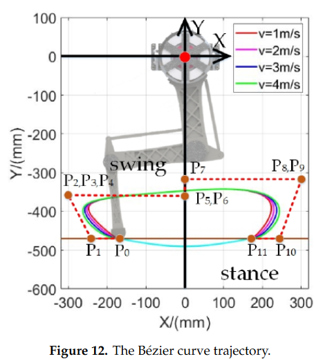
So building a parametric bezier curve (11 points for now) you can follow a closed step loop, i drew this curve on this bezier curve generator: https://www.desmos.com/calculator/xlpbe9bgll

This can by written by an equation dependant of the N point and a parameter going from 0 to 1 in order to describe the trajectory. Here i show you the parametrized Bezier curve:

In the the gaitPlanner.py file t is known as phi. This parameter is important, because it tells you where the foot is located, these coordinates are defined inside the foot frame.

The Points are based on the paper Leg Trajectory Planning for Quadruped Robots with High-Speed Trot Gait from the MIT cheetah robot (equations 11-23-24-TABLE II).

But in my case, i chose similar points but with 10 points (removing P6 and P4) and i'm just multiplying all points by a velocity command in order to make the trajectory wider. This way i have a very simple solution to the stance and swing controller.

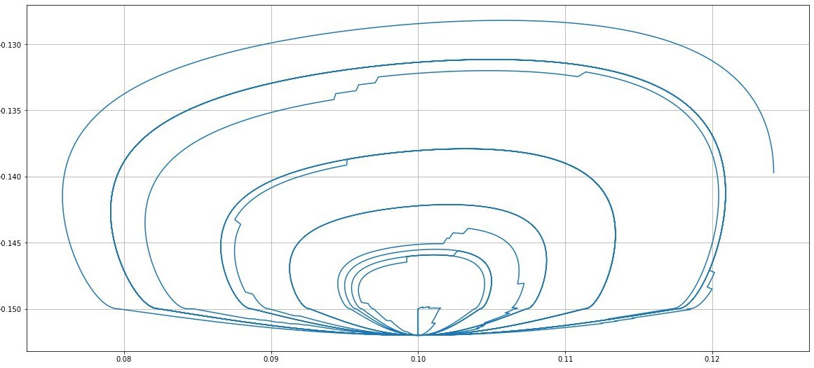
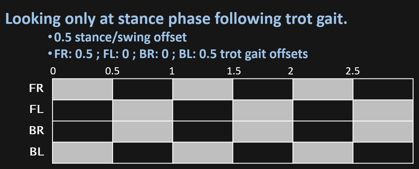
Also for every loop, the swing and stance loops are running, each from 0 to 1, first stance phase then swing, with an offset between them which, if it is set at 0.5, both phases last the same. In another case, for creep gait, this offset must be set at 0.75, meaning that stance phase will last 3/4 of the step.

The code for each leg goes as follow, where most of the code is just to define the signs of vectors needed for the rotation steps as this is defines inside cylindrical coordinates.

def stepTrajectory(self , phi , V , angle , Wrot , centerToFoot): #phi belong [0,1), angles in degrees
        if (phi >= 1):
            phi = phi - 1.


"""
step describes a circuference in order to rotate,
makes the step plane to be inside a circunference.
"""
        r = np.sqrt(centerToFoot[0]**2 + centerToFoot[1]**2) #radius of the ciscunscribed circle
        footAngle = np.arctan2(centerToFoot[1],centerToFoot[0]) 
        
        if Wrot >= 0.:#As it is defined inside cylindrical coordinates, when Wrot < 0, this is the same as rotate it 180ª
            circleTrayectory = 90. - np.rad2deg(footAngle - self.alpha)
        else:
            circleTrayectory = 270. - np.rad2deg(footAngle - self.alpha)
        
"""
then calculate the coordinates to follow the step trajectory
for both ongitudinal and rotational steps.
Here is where the offset between STANCE and SWING is defined. 
"""
        stepOffset = 0.5
        if phi <= stepOffset: #stance phase
            phiStance = phi/stepOffset
            stepX_long , stepY_long , stepZ_long = self.calculateStance(phiStance , V , angle)#longitudinal step
            stepX_rot , stepY_rot , stepZ_rot = self.calculateStance(phiStance , Wrot , circleTrayectory)#rotational step

        else: #swing phase
            phiSwing = (phi-stepOffset)/(1-stepOffset)
            stepX_long , stepY_long , stepZ_long = self.calculateBezier_swing(phiSwing , V , angle)#longitudinal step
            stepX_rot , stepY_rot , stepZ_rot = self.calculateBezier_swing(phiSwing , Wrot , circleTrayectory)#rotational step

"""
define the sign of every cuadrant, angle at which the foot is located,
which is saved in order to know the last position of the rotational step.
"""
        if (centerToFoot[1] > 0): 
            if (stepX_rot < 0):
                self.alpha = -np.arctan2(np.sqrt(stepX_rot**2 + stepY_rot**2) , r)
            else:
                self.alpha = np.arctan2(np.sqrt(stepX_rot**2 + stepY_rot**2) , r)   
        else:
            if (stepX_rot < 0):
                self.alpha = np.arctan2(np.sqrt(stepX_rot**2 + stepY_rot**2) , r)
            else:
                self.alpha = -np.arctan2(np.sqrt(stepX_rot**2 + stepY_rot**2) , r)   

        coord = np.empty(3)        
        coord[0] = stepX_long + stepX_rot
        coord[1] = stepY_long + stepY_rot
        coord[2] = stepZ_long + stepZ_rot
        
        return coord  

Then making 4 loops going from 0 to 1, for every leg and define an offset for every foot you can do different gaits, here is the code:

if (self.phi >= 0.99):
    self.lastTime= time.time()

self.phi = (time.time()-self.lastTime)/T
"""
now it calculates step trajectory for every foot
each step_coord is defined inside the feet frame.
"""
step_coord = self.stepTrajectory(self.phi + offset[0] , V , angle , Wrot , np.squeeze(np.asarray(bodytoFeet_[0,:]))) #FR
self.bodytoFeet[0,0] =  bodytoFeet_[0,0] + step_coord[0]
self.bodytoFeet[0,1] =  bodytoFeet_[0,1] + step_coord[1] 
self.bodytoFeet[0,2] =  bodytoFeet_[0,2] + step_coord[2]
    
step_coord = self.stepTrajectory(self.phi + offset[1] , V , angle , Wrot , np.squeeze(np.asarray(bodytoFeet_[1,:])))#FL
self.bodytoFeet[1,0] =  bodytoFeet_[1,0] + step_coord[0]
self.bodytoFeet[1,1] =  bodytoFeet_[1,1] + step_coord[1]
self.bodytoFeet[1,2] =  bodytoFeet_[1,2] + step_coord[2]
        
step_coord = self.stepTrajectory(self.phi + offset[2] , V , angle , Wrot , np.squeeze(np.asarray(bodytoFeet_[2,:])))#BR
self.bodytoFeet[2,0] =  bodytoFeet_[2,0] + step_coord[0]
self.bodytoFeet[2,1] =  bodytoFeet_[2,1] + step_coord[1]
self.bodytoFeet[2,2] =  bodytoFeet_[2,2] + step_coord[2]

step_coord = self.stepTrajectory(self.phi + offset[3] , V , angle , Wrot , np.squeeze(np.asarray(bodytoFeet_[3,:])))#BL
self.bodytoFeet[3,0] =  bodytoFeet_[3,0] + step_coord[0]
self.bodytoFeet[3,1] =  bodytoFeet_[3,1] + step_coord[1]
self.bodytoFeet[3,2] =  bodytoFeet_[3,2] + step_coord[2]

return self.bodytoFeet

  In order to ilustrate this, here is a diagram which shows the stance face in gray along phi for each foot.

In the video i explain how you can generate different gaits just by changing the offset between the feet loop:

You can play with the simulation at the walking_simulation_example.py file just python3 with pybullet and numpy needed to run the simulation.

In this first log i'm going to explain how the kinematic model works.

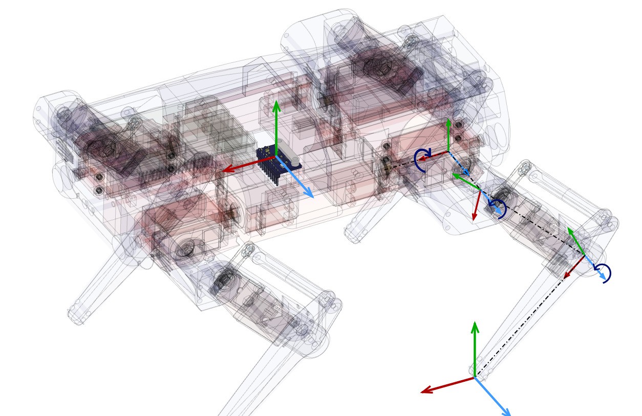
First thing to take into account is the robot geometry and its DOFs, to ilustrate this, in the next image you see where are they and how they transform. This model is very looking forward, in real robotics first is to make a robust state stimator so you can have smooth meassurements of robots states.

NOTE: All vector are defined inside the robot frame, no world frame is used for now.

So, we have 4 frames on each leg and one which is commun for all, which is the geometric center of the robot (very close to the CoM).

For our setup, there are 2 important frames on the leg, which are the frame0 (coxa frame or first frame on the leg) and frame4 (foot frame or last frame on the leg).

So now, we are going to calculate Inverse Kinematics between those frames. If you want more information on how to calculate IK you can read this article: https://www.researchgate.net/publication/320307716_Inverse_Kinematic_Analysis_Of_A_Quadruped_Robot

As u can see the setup is a bit diferent, but it only change the simetry of the legs, so the analytic function is the same.

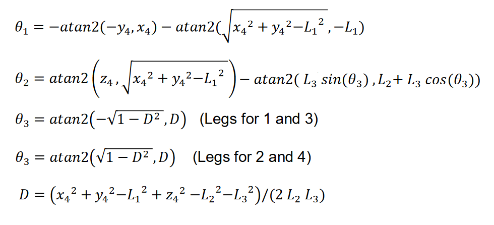
Inverse Kinematics are solved on the IK_solver.py file, which is basically two functions, one for right legs and the other for the left legs. These functions works as shown:

And the code goes as follow:

def solve_R(coord , coxa , femur , tibia): 
"""where:
   coord = np.array([x4,y4,z4])
   coxa = L1 
   femur = L2 
   tibia = L3
"""
    D = (coord[1]**2+(-coord[2])**2-coxa**2+(-coord[0])**2-femur**2-tibia**2)/(2*tibia*femur)  
    D = checkdomain(D) #This is just to deal with NaN solutions
    gamma = numpy.arctan2(-numpy.sqrt(1-D**2),D)
    tetta = -numpy.arctan2(coord[2],coord[1])-numpy.arctan2(numpy.sqrt(coord[1]**2+(-coord[2])**2-coxa**2),-coxa)
    alpha = numpy.arctan2(-coord[0],numpy.sqrt(coord[1]**2+(-coord[2])**2-coxa**2))-numpy.arctan2(tibia*numpy.sin(gamma),femur+tibia*numpy.cos(gamma))
    angles = numpy.array([-tetta, alpha, gamma])
    return angles

 Now, we can locate foot in the 3D space, inside the frame0.

Next step is to move the body frame in relation with the feet. Which is essentialy the kinematic model i built, kinematic_model.py file in the code.

For this, we need to define 3 vectors, the vector from the center to the frame0 or coxa frame is going to be rotated and translated with the desired body position.

The next is the vector from body frame to frame4 or foot frame, this vector is where we want the foot to stay with recpect to world coordinates.

With this two vector we can calculate the IK vector needed for the inverse kinematics just by subtracting body to frame4 and body to frame0.

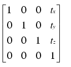
Now, we want the body to rotate on its 3 dofs and its 3 logitudinal movements, for this, we just multiply the body to frame0 vector by the rototranslation matrix, shown at the next step:

You can see how this woks on the geometrics.py file, where the fuctions for the rototranslations are defined. You only need to multiply these matrix by the vector you want to transform:

def RTmatrix(orientation, position):
    """compose translation and rotation"""
    roll = orientation[0]
    pitch = orientation[1]
    yaw = orientation[2]
    x0 = position[0]
    y0 = position[1]
    z0 = position[2]
    
    translation = np.matrix([[1, 0, 0, x0],#Translation matrix
                             [0, 1, 0, y0],
                             [0, 0, 1, z0],
                             [0, 0, 0,  1]])
    rotation = Rxyz(roll, pitch, yaw)#rotation matrix
    
    return rotation*translation
    
def transform(coord,rotation,translation):
    """transforms a vector to a desire rotation and translation"""
    vector = np.array([[coord[0]],
                       [coord[1]],
                       [coord[2]],
                       [      1]])
    
    tranformVector = RTmatrix(rotation,translation)*vector
    return np.array([tranformVector[0,0], tranformVector[1,0], tranformVector[2,0]])

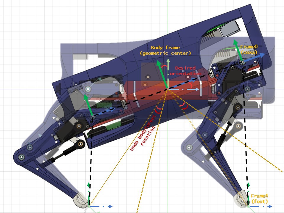
Here there is a figure to ilustrate the rotation of the body with respect to the feet in the pitch rotation:

As the the principal frame is transformed, all other child frames are also transformed,  so in order to keep feet still, we need to undo the fransformation for the frame0 to frame4 vector (IK vector) before IK are solved. This ends with all frames transformed in order to mantein the the frame4 at the same position with respect the BodyFrame.

Here is the code solving that:

    def solve(self, orn , pos , bodytoFeet):
        bodytoFR4 = np.asarray([bodytoFeet[0,0],bodytoFeet[0,1],bodytoFeet[0,2]])
        bodytoFL4 = np.asarray([bodytoFeet[1,0],bodytoFeet[1,1],bodytoFeet[1,2]])
        bodytoBR4 = np.asarray([bodytoFeet[2,0],bodytoFeet[2,1],bodytoFeet[2,2]])
        bodytoBL4 = np.asarray([bodytoFeet[3,0],bodytoFeet[3,1],bodytoFeet[3,2]])

        """defines 4 vertices which rotates with the body"""
        _bodytoFR0 = geo.transform(self.bodytoFR0 , orn, pos)
        _bodytoFL0 = geo.transform(self.bodytoFL0 , orn, pos)
        _bodytoBR0 = geo.transform(self.bodytoBR0 , orn, pos)
        _bodytoBL0 = geo.transform(self.bodytoBL0 , orn, pos)
        """defines coxa_frame to foot_frame leg vector neccesary for IK"""
        FRcoord = bodytoFR4 - _bodytoFR0
        FLcoord = bodytoFL4 - _bodytoFL0
        BRcoord = bodytoBR4 - _bodytoBR0
        BLcoord = bodytoBL4 - _bodytoBL0
        """undo transformation of leg vector to keep feet still"""
        undoOrn = -orn
        undoPos = -pos
        _FRcoord = geo.transform(FRcoord , undoOrn, undoPos)
        _FLcoord = geo.transform(FLcoord , undoOrn, undoPos)
        _BRcoord = geo.transform(BRcoord , undoOrn, undoPos)
        _BLcoord = geo.transform(BLcoord , undoOrn, undoPos)
        
        """solve inverse kinematics with frame0 to frame4 vector"""
        FR_angles = IK.solve_R(_FRcoord , self.coxa , self.femur , self.tibia)
        FL_angles = IK.solve_L(_FLcoord , self.coxa , self.femur , self.tibia)
        BR_angles = IK.solve_R(_BRcoord , self.coxa , self.femur , self.tibia)
        BL_angles = IK.solve_L(_BLcoord , self.coxa , self.femur , self.tibia)
        
        _bodytofeetFR = _bodytoFR0 + _FRcoord
        _bodytofeetFL = _bodytoFL0 + _FLcoord
        _bodytofeetBR = _bodytoBR0 + _BRcoord
        _bodytofeetBL = _bodytoBL0 + _BLcoord
        _bodytofeet = np.matrix([[_bodytofeetFR[0] , _bodytofeetFR[1] , _bodytofeetFR[2]],
                                 [_bodytofeetFL[0] , _bodytofeetFL[1] , _bodytofeetFL[2]],
                                 [_bodytofeetBR[0] , _bodytofeetBR[1] , _bodytofeetBR[2]],
                                 [_bodytofeetBL[0] , _bodytofeetBL[1] , _bodytofeetBL[2]]])
        
        return FR_angles, FL_angles, BR_angles, BL_angles , _bodytofeet

 Here there is a video showing the model in action:

As you see in the video, you can define a initial position for the feet and vary the 6 dof on the body frame, that it may be, for example, the states of a control model.