Acoustic Source Localization

Once again, the writing for this log is taken directly from an engineering analysis I wrote. This post goes over the equations and simulation results of the hydrophone array. I’ll likely add further simulation results later on.

*from engineering analysis*

The MATLAB simulation will model the fundamental aspects of the hydrophone array solution. This simulation needs to model the acoustic propagation, analog signal conditioning, signal discretization, and the microprocessor algorithm. Using this model, the true target location can be compared to the decoded location, allowing for an analysis of system accuracy, noise tolerance, and computation time. Furthermore, this simulation will provide a clear path for firmware development and finalizes the technical feasibility of the design.

When in water, sound waves travel at a variable speed described by equation (2.1) [3]. This equation depends on the water temperature in Celsius, T, water salinity in parts per thousand, S, and the depth below the surface in meters, D.

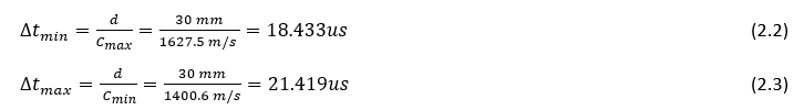
Although the speed of sound is variable, it would help simplify both hardware and firmware design if it could be assumed constant. To gauge the effect of this assumption, equation (2.1) was tested over the range of feasible inputs. When temperature is varied from 0 to 30’C, depth 0 to 50m, and salinity 0 to 35 ppm. The resulting maximum and minimum speeds are 1647.6 meters per second, and 1400.6 meters per second using equation (2.1). Assuming the transducers are separated by 30 millimeters, which is the case for AUVIC’s hydrophone enclosure, the largest propagation delay would result when the target is 90 degrees, or perpendicular, to the AUV’s direction of travel. In this case the time difference of arrivals between the two signals would be at maximum 7.1 microseconds, and at minimum 6.1 microseconds shown in equation (2.2) and (2.3); where, d, is the distance between hydrophones, and, C, is the speed of sound.

Assuming the ADC samples the signal at 100 thousand samples per second (KSPS), this variability will marginally affect the overall accuracy of the system. Furthermore, regardless of the overall accuracy measurements, the algorithm will naturally approach the true location based on the AUV’s movement. For example, assume that every decoded trajectory has an error of 25 percent. After each course adjustment, the AUV comes closer to the target, hence the overall accuracy becomes less and less of a concern. Eventually the AUV will be close enough to the target for the AUV’s optics to take over. For these reasons, the speed of sound in water will be treated as a constant of 1500 meters per second for all subsequent analyses.

Next consider the phase difference of the received signals. The formula to convert this phase shift to the angle of arrival is presented in equation (2.4). This formula is derived from illustration in Figure 1; where, theta, is the direction to the target or angle of arrival, delta t, is the time difference of arrival between the two received signals, and, C, is the speed of sound on water.

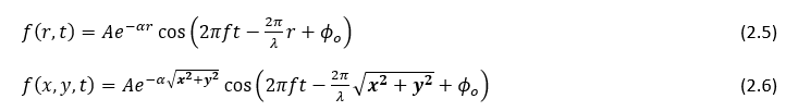
Next consider an acoustic wave traveling on a 2D plane as described by equation (2.5) [4]. This formula relates the amplitude of a signal over position and time, where A, is the sending end amplitude, a, is the attenuation constant, f, is the frequency, t, is the time, lambda, is the wavelength, r, is the distance from the emitter to the receiver, and, phi, is the initial phase shift of the signal. For the purposes of this report the equation was modified to incorporate the cartesian coordinate system by making the substitution r=sqrt(x^2+y^2). The modified equation is shown in equation (2.6).

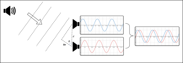
Equation (2.6) was then translated to MATLAB, and two hydrophones were placed on arbitrary points on the waveforms surface, seperated by 2cm. The hydrophones are represented by the red and blue dots in the upper image of Figure 3. As seen in Figure 3 the signals received by the hydrophones (bottom stem plot representing ADC samples) are phase shifted copies of one another.

The following theory of operation is taken from my engineering analysis (separate document). It might sound a bit awkwardly formal for these logs, but it explains the concept of this design pretty well… and I don’t want to rewrite the theory of operation : ) .

*From engineering analysis*

To understand the theory of operation, consider a small hydrophone array consisting of two hydrophones separated by a known distance (d), shown in Figure 1. These hydrophones receive acoustic pressure waves from an un-identified “target” and convert them to weak electrical signals via a piezoelectric transducer [1]. Depending on the position of the target, the signals received by the hydrophones will be identical, although phase shifted, copies of one another. If the acoustic propagation constant is known, then this phase shift can be directly related to the angle of arrival of the incoming plane wave.

There are several assumptions that need to be considered when implementing this model. Foremost, this model assumes the propagation speed is known and constant; however, this parameter depends on the water temperature, water depth, and water salinity [3]. Next, consider the 2D model in Figure 1, if the illustration is extrapolated to a 3D space, the solution would have a cone of solutions at angle. Even this 2D model leads to an extraneous root symmetric about the two hydrophones. Lastly, the angle of arrival assumption requires a plane wave. For this assumption to be appropriate, the distance from the target to the hydrophone must be much greater than the distance (d) between the hydrophones.

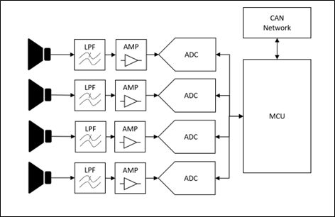
Implementing the solution on hardware is feasible based on existing systems used on various AUV’s such as [2]. There are many methods to implement this system on hardware, so only a generalized overview will be provided. The block diagram is shown in Figure 2, and consists of an analog front end for filtering and amplification of the incoming signal, an analog to digital converter (ADC) to discretize the waveform, and a microprocess to interpret the results.

The University of Victoria’s Autonomous Underwater Vehicle (AUV) club AUVIC, competes in a yearly RoboSub competition. During this competition, the clubs’ AUV completes several tasks outlined by the RoboSub committee; such as collecting markers and using computer vision to decipher images. To navigate between these tasks the AUV needs to follow several acoustic beacons placed around the course.

A subsystem is needed to interpret the direction or location of these acoustic “pings” (momentary single frequency pressure wave emitted from the beacons) and communicate this information to the main “Trident” AUV. This data needs to be communicated within reasonable accuracy (< ~30⁰) and time (< ~2 seconds processing time); and must be accomplished within AUVIC’s budget.

This system will use one of the following solutions to calculate the expected location/direction of the beacons. The PCBA (Printed Circuit Board Assembly) will be designed to allow for either solution to be implemented.

Solution 1: Using a single hydrophone and an inertial measurement unit (IMU), a basic location can be calculated by observing the change in signal amplitude over time.

(SELECTED) Solution 2: Using a 4-hydrophone array it’s possible to calculate the position of an acoustic emitter based on the phase shift of the signal between each hydrophone or based on the signals’ time difference of arrival. This assumes the hydrophone locations are known and the speed of sound in water can be reasonably approximated.